Lexiton International
Lexiton International Welcome to Lexiton International
Level 6 Diploma in Quality Assurance and Quality Control (QA/QC) Mechanical
Section 1: Unit 1: Advanced Quality Management Systems in Mechanical Engineering
Section 2: Unt No 2: Mechanical System Inspection and Testing Techniques
Section 3: Unit 3: Statistical Process Control and Data Analysis in Mechanical Engineering
Lesson 1:Apply statistical methods to monitor and control mechanical engineering and manufacturing processes. Quiz No 1: Apply statistical methods to monitor and control mechanical engineering and manufacturing processes. Lesson 2: Collect, analyse, and interpret mechanical data to support QA/QC decision-making. Quiz No 2: Collect, analyse, and interpret mechanical data to support QA/QC decision-making. Lesson 3: Identify trends, variations, and potential issues in mechanical quality and performance. Quiz No 3: Identify trends, variations, and potential issues in mechanical quality and performance. Lesson 4: Use data-driven strategies to improve process efficiency and component reliability. Quiz No 4: Use data-driven strategies to improve process efficiency and component reliability. Lesson 5: Implement control charts, KPIs, and performance metrics to maintain high-quality standards. Quiz No 5: Implement control charts, KPIs, and performance metrics to maintain high-quality standards. Lesson 6: Support continuous improvement initiatives through precise and actionable data analysis. Quiz No 6: Support continuous improvement initiatives through precise and actionable data analysis.
Section 4: Unit No 4: Mechanical Components, Materials, and Reliability in QA/QC
Section 5: Unit no 5 : Compliance with International Mechanical Standards and Regulations
Section 6: Unit no 6 :Leadership, Risk Management, and Project Supervision in QA/QC Mechanical
Lesson 18

Lesson 6: Support continuous improvement initiatives through precise and actionable data analysis.

Continuous improvement in mechanical engineering and manufacturing depends on the ability to transform reliable quality data into precise, timely and actionable engineering decisions. Lesson 6, “Support continuous improvement initiatives through precise and actionable data analysis,” focuses on how inspection results, process measurements, defect records, performance indicators and historical quality information can be systematically analysed to identify improvement opportunities. Effective data analysis enables QA/QC teams and engineering professionals to move beyond simply recording defects and instead understand why performance changes, where process weaknesses occur and which interventions are most likely to deliver measurable improvement.

In modern mechanical manufacturing environments, data-driven continuous improvement supports better process stability, component reliability, production efficiency and quality performance. Statistical trends, control-chart information, inspection results, rejection patterns, rework records and key performance indicators can provide evidence for identifying recurring problems and evaluating the effectiveness of corrective actions. By interpreting these sources accurately, engineering teams can distinguish significant process changes from normal variation, prioritise improvement opportunities and establish measurable improvement objectives. This approach strengthens evidence-based decision-making across machining, fabrication, welding, assembly, inspection and mechanical quality-control activities while helping organisations maintain consistent engineering and quality standards.

The lesson also examines how precise data analysis can be converted into practical improvement actions. Rather than treating data as a historical record, effective QA/QC practice uses it as a feedback mechanism for process optimisation, defect prevention and performance improvement. Engineers can use validated information to identify root causes, compare pre- and post-improvement performance, monitor corrective-action effectiveness and determine whether improvements have been sustained. From a broader quality-management perspective, this supports a structured cycle of measurement, analysis, intervention, verification and continual improvement. The result is a more reliable and responsive mechanical engineering environment in which decisions are supported by objective evidence, quality risks are addressed proactively and improvement initiatives can be demonstrated through measurable performance outcomes.

1 Formulate clear, data-backed problem statements that highlight specific areas of inefficiency or high defect rates within mechanical operations

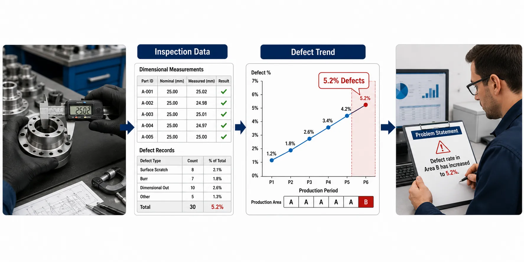
In mechanical engineering, manufacturing and QA/QC environments, effective continuous improvement begins with correctly defining the problem. A poorly defined problem can cause engineering teams to investigate the wrong process, collect irrelevant information, apply ineffective corrective actions or spend resources on symptoms rather than causes. A clear, data-backed problem statement provides a factual starting point for improvement by describing what is happening, where it is happening, how frequently it occurs, how significant the effect is and how current performance differs from the expected condition. The purpose is not to identify the cause prematurely, but to establish an objective description of the performance gap that can subsequently be investigated using appropriate engineering and quality-analysis techniques.

For a mechanical engineering professional, formulating a problem statement requires the integration of inspection data, production records, defect reports, process measurements, rejection statistics, rework information, equipment performance records and other relevant evidence. The statement should distinguish verified facts from assumptions and should identify the measurable difference between current and required performance. This creates a reliable foundation for subsequent root-cause analysis, process improvement, corrective action and verification. Whether the issue concerns dimensional variation in machining, excessive welding defects, repeated assembly failures, material waste, extended cycle times or increasing component rejection, the quality of the problem statement directly influences the quality of the improvement process.

Understanding a data-backed problem statement

A data-backed problem statement is a concise, evidence-based description of a defined performance problem supported by verified quantitative or qualitative information.

It should answer fundamental questions such as:

  • What is the problem?
  • Where is it occurring?
  • When is it occurring?
  • How frequently does it occur?
  • How large is the performance gap?
  • Which component, process or operation is affected?
  • What requirement or target is not being achieved?
  • What measurable impact is being created?
  • What evidence confirms that the problem exists?

A strong problem statement does not normally state an unverified root cause.

For example:

Weak statement:

“Operators are producing poor-quality components because they are not following the process.”

This contains assumptions about the cause.

A stronger statement is:

“Dimensional rejection of machined shafts increased from 1.8% to 4.6% over six production weeks, with 72% of recorded dimensional defects occurring at the final turning operation.”

The second statement is supported by measurable evidence and identifies a specific area requiring investigation without prematurely claiming why the problem exists.

The role of problem definition in continuous improvement

Continuous improvement follows a logical sequence in which the problem must be understood before solutions are selected.

A simplified sequence is:

Problem identification → Data validation → Problem definition → Root-cause analysis → Improvement action → Verification → Standardisation

If the first stage is weak, subsequent stages may also become unreliable.

A well-defined problem statement helps the engineering team:

  • Establish a common understanding of the issue.
  • Define the scope of investigation.
  • Identify the data required.
  • Select appropriate analytical methods.
  • Prioritise improvement activities.
  • Establish measurable objectives.
  • Avoid premature conclusions.
  • Compare performance before and after intervention.
  • Communicate the issue to management and production teams.

Key concepts in data-backed problem formulation

ConceptDefinitionMechanical engineering application
Problem statementFactual description of a defined performance gapIncreased dimensional rejection on a machining line
Performance gapDifference between actual and required performanceRejection rate above the approved target
BaselineValid reference point for comparisonAverage defect rate before improvement
Defect rateProportion of inspected items containing defined defectsPercentage of components with dimensional deviations
Rejection ratePercentage of inspected items rejected against acceptance criteriaRejected machined components
Rework ratePercentage or quantity requiring additional processingComponents requiring corrective machining
Cycle timeTime required to complete a defined operationAssembly time per mechanical unit
EfficiencyRelationship between resources used and useful outputProduction output relative to operating time
TrendPattern of performance change over timeIncreasing bearing-seat dimensional deviation
EvidenceVerified information supporting a conclusionInspection records and measured values
ScopeDefined boundaries of the investigationSpecific machine, product or production shift
Root causeUnderlying factor responsible for an identified problemTool wear causing dimensional drift
ContainmentImmediate action limiting the impact of a detected problemSegregating potentially affected components
Corrective actionAction intended to eliminate the cause of a non-conformityRevising tooling control after verified root cause
Improvement objectiveDefined measurable result expected from an interventionReducing rejection from 4.6% to below 2%

Difference between a problem statement and a root-cause statement

This distinction is fundamental to professional QA/QC practice.

A problem statement describes the observed condition.

A root-cause statement explains why the condition occurred.

For example:

Problem statement:

“Welded assemblies recorded a 7.2% defect rate during the previous month, compared with the established target of 3%.”

Potential root-cause statement:

“Variation in welding parameters contributed to the increased defect rate.”

The second statement should only be adopted after appropriate investigation and evidence confirm the relationship.

Prematurely placing a suspected cause into the problem statement can introduce confirmation bias and cause the investigation team to overlook alternative explanations.

Characteristics of an effective problem statement

A professional problem statement should generally be:

  • Specific.
  • Evidence-based.
  • Measurable.
  • Relevant.
  • Time-bound.
  • Clearly scoped.
  • Neutral.
  • Traceable.
  • Understandable.
  • Action-oriented without prescribing an unverified solution.

It should avoid vague expressions such as:

  • “Quality is poor.”
  • “Production is too slow.”
  • “The machine is unreliable.”
  • “Operators are making mistakes.”
  • “The process needs improvement.”

These statements may identify a concern but do not provide enough evidence to support systematic investigation.

Using the SMART principle

A useful approach is to make problem statements specific, measurable, relevant and time-defined.

For example:

“During the last eight production weeks, the machining cell recorded an average dimensional rejection rate of 5.1%, compared with the approved target of 2.0%, with the majority of defects associated with shaft diameter measurements.”

This statement identifies:

  • Time period.
  • Process area.
  • Current performance.
  • Expected performance.
  • Defect characteristic.

Establishing the performance baseline
Four Step Quality Control Process

Before formulating a problem statement, the engineer should establish a reliable baseline.

A baseline provides the reference against which deterioration or improvement can be assessed.

Potential baseline information includes:

  • Historical rejection rate.
  • Average dimensional deviation.
  • First-pass acceptance.
  • Rework percentage.
  • Cycle time.
  • Material waste.
  • Equipment downtime.
  • Defect frequency.
  • Customer complaints.
  • Inspection results.

The baseline should be representative of the process being investigated.

Validating the data before defining the problem

A problem statement is only as reliable as its supporting data.

Before using data, QA/QC personnel should examine:

  • Data completeness.
  • Measurement accuracy.
  • Correct units.
  • Correct component identification.
  • Correct drawing revision.
  • Inspection method.
  • Equipment calibration status.
  • Sampling approach.
  • Date and time.
  • Production batch.
  • Operator or workstation information where relevant.
  • Duplicate records.
  • Missing records.

If the underlying data is unreliable, the problem statement may describe a data-quality problem rather than an actual manufacturing problem.

Example of data validation

A production report indicates that dimensional rejection increased from 2% to 8%.

Before declaring major process deterioration, the engineer discovers that:

  • The inspection sample size doubled.
  • A more sensitive measurement method was introduced.
  • The specification was unchanged.

The apparent increase may therefore require additional analysis before being described as a genuine eight-percent process failure.

A more appropriate problem statement might recognise the change in inspection coverage and compare equivalent datasets.

Defining the scope

The scope determines exactly where the problem exists.

A mechanical operation may include:

  • Multiple machines.
  • Multiple shifts.
  • Different products.
  • Different materials.
  • Multiple tooling configurations.
  • Several inspection stages.

A statement such as “machining quality has deteriorated” is too broad.

A better statement may identify:

  • One machining cell.
  • One component family.
  • One dimensional characteristic.
  • A defined production period.

This prevents investigation resources from being unnecessarily distributed across unrelated processes.

Identifying inefficiency

Not all continuous improvement problems involve product defects.

Inefficiency may occur through:

  • Excessive cycle time.
  • Unnecessary movement.
  • Excessive inspection time.
  • Material waste.
  • Repeated setup activities.
  • Excessive machine downtime.
  • Rework.
  • Waiting time.
  • Duplicate documentation.
  • Unbalanced workflow.
  • Poor resource utilisation.

The problem statement should quantify the inefficiency where possible.

For example:

“Average mechanical assembly cycle time increased from 42 minutes to 58 minutes over six weeks, resulting in an estimated 27% reduction in hourly output.”

This is significantly more useful than saying:

“Assembly is taking too long.”

Identifying high defect rates

A high defect rate should be clearly defined in relation to a reference point.

For example:

“Bearing housing dimensional defects increased to 6.4% during May compared with the established 2.5% target.”

The statement can then be further scoped:

“Of the recorded defects, 68% were associated with bore diameter measurements.”

This helps the team identify where analytical effort should be concentrated.

Separating symptoms from the problem

A symptom is an observable effect.

A problem statement should describe the performance condition without automatically assuming its cause.

For example:

Symptom:

“Components are being rejected.”

Better problem statement:

“Component rejection increased from 2.1% to 5.7% during the previous six weeks, with dimensional defects accounting for 64% of all recorded rejections.”

Potential causes may include:

  • Tool wear.
  • Fixture movement.
  • Measurement error.
  • Material variation.
  • Machine instability.
  • Incorrect process settings.

These causes should be investigated rather than assumed.

Using Pareto information

Pareto analysis can help identify the most significant contributors to a quality problem.

Suppose a fabrication department records 500 defects:

  • Weld porosity: 190.
  • Dimensional deviation: 140.
  • Surface damage: 80.
  • Incorrect assembly: 50.
  • Missing documentation: 40.

The problem statement may focus on the dominant defect categories rather than treating every defect as equally significant.

For example:

“Weld porosity and dimensional deviation account for 66% of recorded fabrication defects during the current quarter, indicating a concentrated opportunity for process improvement.”

Using trend data

A single measurement may indicate an event, but a trend can reveal a developing process problem.

For example:

WeekRejection Rate
11.9%
22.1%
32.4%
42.8%
53.3%
63.9%

A problem statement based on the trend could state:

“Dimensional rejection has increased progressively from 1.9% to 3.9% over six weeks, indicating a sustained deterioration requiring process investigation.”

This is stronger than simply reporting the latest 3.9% value.

Using control-chart information

Where statistical process control is used, control charts can strengthen problem definition.

Relevant evidence may include:

  • Points outside control limits.
  • Sustained runs.
  • Trends.
  • Increasing ranges.
  • Shifts in process average.
  • Changes in process variation.

For example:

“Eight consecutive subgroup averages have shifted above the established process centre line, coinciding with an increase in dimensional rejection.”

This provides a statistically informed description of the issue.

Connecting problem statements with KPIs

Existing KPIs can provide valuable evidence.

Relevant indicators may include:

  • Rejection rate.
  • First-pass acceptance.
  • Rework rate.
  • Inspection cycle time.
  • Quality escape rate.
  • Defects per batch.
  • Corrective-action closure time.
  • Material waste.
  • Equipment downtime.

A problem statement should use the KPI most directly connected to the observed performance gap.

Using multiple data sources

Complex mechanical problems often require evidence from multiple sources.

For example, an assembly reliability problem may require:

  • Inspection results.
  • Maintenance logs.
  • Production records.
  • Component failure reports.
  • Vibration data.
  • Temperature records.
  • Rework records.

If multiple sources demonstrate the same pattern, confidence in the problem definition increases.

Practical example: machining inefficiency

A CNC machining cell reports declining output.

Initial statement:

“The CNC machine is too slow.”

Data collection identifies:

  • Standard cycle time: 12 minutes.
  • Current average: 16 minutes.
  • Setup interruptions: 3 per shift.
  • Tool-change delays: 22 minutes per shift.
  • Rework associated with dimensional drift: 3.8%.

A stronger problem statement becomes:

“The CNC machining cell is averaging 16 minutes per component against a 12-minute standard, while tool-change delays and dimensional rework contribute to recurring production losses.”

The team can now investigate the relevant factors.

Practical example: welding defects

A fabrication department experiences increased rejection.

Collected data shows:

  • Previous rejection rate: 2.4%.
  • Current rejection rate: 6.1%.
  • 71% of defects involve weld porosity.
  • 64% of porosity defects originate from one welding station.

A suitable problem statement could be:

“Welding rejection at the fabrication department has increased from 2.4% to 6.1%, with porosity accounting for 71% of defects and 64% of porosity cases originating from one welding station.”

This gives the investigation team a clear direction without claiming the cause.

Practical example: mechanical assembly rework

An assembly line experiences increasing rework.

Data reveals:

  • Rework rate increased from 3% to 7%.
  • 55% of rework concerns alignment.
  • 70% of alignment rework occurs at one workstation.
  • The problem began after a recent production change.

A data-backed statement could be:

“Assembly rework has increased from 3% to 7%, with alignment-related work representing 55% of rework and 70% of alignment cases occurring at one workstation following a recent process change.”

This provides a strong basis for subsequent investigation.

Practical example: material waste

A mechanical fabrication team identifies excessive material consumption.

Historical data shows:

  • Planned material utilisation: 92%.
  • Current utilisation: 83%.
  • Scrap increased by 18%.
  • Scrap concentration is highest in one component family.

A suitable statement could be:

“Material utilisation has declined from the planned 92% to 83%, with an 18% increase in scrap concentrated within one component family during the current production period.”

The engineering team can then investigate cutting patterns, material preparation, dimensional requirements and process conditions.

Distinguishing fact from interpretation

A high-quality problem statement uses factual language.

Prefer:

“Inspection records show a 4.8% rejection rate.”

Avoid:

“The inspection team is failing to control quality.”

Prefer:

“Rework increased by 22% following the process change.”

Avoid:

“The new process is poorly designed.”

The first versions can be verified through evidence.

Establishing problem magnitude

A problem should be quantified wherever possible.

Useful measures include:

  • Percentage.
  • Quantity.
  • Frequency.
  • Time.
  • Cost.
  • Rate.
  • Deviation.
  • Downtime.
  • Waste.
  • Customer impact.

For example:

“Three hundred and forty components required rework during the quarter, representing 6.8% of total production.”

This is more informative than:

“Many components required rework.”

Identifying the affected process stage

A mechanical operation should be broken into relevant stages.

For machining:

  • Material preparation.
  • Workholding.
  • Rough machining.
  • Finishing.
  • Tool change.
  • Measurement.
  • Final inspection.

For assembly:

  • Component preparation.
  • Positioning.
  • Fastening.
  • Alignment.
  • Torque application.
  • Functional verification.
  • Final inspection.

The problem statement should identify the stage where the performance gap is concentrated when the evidence supports it.

Linking the problem to requirements

A useful problem statement should compare actual performance with an appropriate requirement.

Possible reference points include:

  • Approved drawing.
  • Client specification.
  • Internal quality target.
  • Production standard.
  • Process capability objective.
  • Contractual requirement.
  • Approved procedure.

For example:

“Dimensional rejection is 4.2%, compared with the approved quality target of 2%.”

This creates a clear performance gap.

Establishing data traceability

Every major figure used in a problem statement should be traceable to its source.

Sources may include:

  • Inspection reports.
  • Non-conformance reports.
  • Production databases.
  • Control charts.
  • Quality dashboards.
  • Maintenance records.
  • Test reports.
  • Measurement-system records.

Traceability allows the engineering team to verify the statement and prevents decisions based on unsupported figures.

Problem statement development process

A structured procedure can be used:

  1. Identify the initial quality or efficiency concern.
  2. Define the process affected.
  3. Collect relevant data.
  4. Validate the data.
  5. Establish the baseline.
  6. Identify applicable requirements.
  7. Quantify the performance gap.
  8. Analyse trends.
  9. Segment the data where appropriate.
  10. Identify the most significant affected areas.
  11. Define the investigation scope.
  12. Draft the problem statement.
  13. Check that assumptions have been removed.
  14. Verify supporting evidence.
  15. Obtain appropriate technical review.
  16. Establish the investigation objective.

Data segmentation

Aggregated data can hide important patterns.

Data may need to be separated by:

  • Machine.
  • Shift.
  • Operator.
  • Component.
  • Material batch.
  • Supplier.
  • Product family.
  • Workstation.
  • Date.
  • Tool.
  • Production line.

For example, an overall rejection rate of 3% may appear manageable. However:

  • Machine A: 1%.
  • Machine B: 1.2%.
  • Machine C: 7.8%.

The problem is clearly concentrated at Machine C.

Avoiding misleading averages

Averages can hide important variation.

Suppose two production lines have:

  • Line A rejection: 1%.
  • Line B rejection: 9%.

The combined average may appear moderate depending on production volume, but Line B may require immediate investigation.

Therefore, engineers should examine:

  • Distribution.
  • Range.
  • Variation.
  • Frequency.
  • Location.
  • Product type.

Using evidence hierarchy

Not all information has equal evidential strength.

A practical hierarchy may be:

  1. Verified inspection measurements.
  2. Validated production records.
  3. Controlled quality records.
  4. Approved test reports.
  5. Statistical analysis.
  6. Verified operator observations.
  7. Engineering observations.
  8. Unverified assumptions.

A professional problem statement should rely primarily on validated evidence.

Common mistakes in problem statements

Blaming personnel

Statements such as “operators are causing defects” should not be used without verified evidence.

Naming an unverified root cause

A problem statement should not assume that tool wear, operator error or material quality is responsible before investigation.

Using vague language

Words such as “many”, “often”, “poor” and “slow” should be replaced with measurable evidence.

Combining unrelated problems

Separate issues should normally be investigated separately unless evidence demonstrates a common relationship.

Ignoring historical context

Current performance should be compared with appropriate historical or required benchmarks.

Using obsolete specifications

The statement should reference the current approved requirement.

Using unvalidated data

Incorrect measurements can result in incorrect problem definition.

Benefits of data-backed problem statements

A robust problem statement supports:

  • More focused investigations.
  • Better engineering decisions.
  • Efficient use of resources.
  • Objective communication.
  • Improved root-cause analysis.
  • Better corrective actions.
  • Stronger QA/QC governance.
  • Improved process control.
  • Reduced defect recurrence.
  • More reliable improvement measurement.
  • Better management reporting.
  • Stronger customer confidence.

Relationship between problem statements and root-cause analysis

Once the problem is clearly defined, appropriate analytical techniques can be selected.

These may include:

  • Pareto analysis.
  • Trend analysis.
  • Control charts.
  • Five Whys.
  • Fishbone analysis.
  • Process mapping.
  • Comparative analysis.
  • Correlation analysis where appropriate.
  • Failure-data analysis.

The problem statement establishes what needs to be explained; root-cause analysis investigates why it occurred.

Linking problem statements with improvement objectives

A well-defined problem should allow the team to establish a measurable improvement objective.

For example:

Problem:

“Dimensional rejection increased to 5.2% against a 2% target.”

Improvement objective:

“Reduce dimensional rejection to below 2% while maintaining required production output and inspection controls.”

This creates a measurable basis for evaluating the effectiveness of improvement actions.

Monitoring the problem after intervention

A problem statement should remain connected to subsequent performance monitoring.

After an intervention, the engineering team should compare:

  • Baseline performance.
  • Post-intervention performance.
  • Defect frequency.
  • Process variation.
  • Rework.
  • Production efficiency.
  • Customer outcomes.

For example:

Before intervention: 5.2% rejection.

After intervention: 2.1%.

Sustained after three months: 1.9%.

This provides stronger evidence that the improvement was effective.

Case Study: Data-backed problem formulation in a precision machining operation

Background

A precision mechanical manufacturing facility produces shafts for industrial equipment. The QA/QC department notices an increase in dimensional rejection during final inspection.

Initial production reports show that rejection has increased during the previous two months.

The production manager initially suggests that the issue is caused by operator technique.

However, the QA/QC engineer does not include this assumption in the problem statement.

Data collection

The team reviews:

  • Final inspection records.
  • Machine-specific rejection data.
  • Shaft diameter measurements.
  • Tool-change records.
  • Production batches.
  • Rework records.
  • Measurement equipment records.
  • Maintenance history.

The analysis identifies:

  • Previous average rejection: 1.7%.
  • Current average rejection: 4.9%.
  • 76% of rejected shafts have diameter-related defects.
  • 68% of diameter defects originate from one machining cell.
  • The increase began approximately five weeks ago.
  • The affected cell has experienced increased tool-change frequency.

Problem statement

The team formulates:

“Dimensional rejection within the shaft production process has increased from an historical average of 1.7% to 4.9% over the previous five weeks. Diameter-related defects account for 76% of rejected components, with 68% of these defects originating from one machining cell.”

This statement is:

  • Specific.
  • Measurable.
  • Traceable.
  • Time-bound.
  • Process-focused.
  • Evidence-based.

It does not claim that tool wear is the cause.

Subsequent investigation

The engineering team can now investigate:

  • Tool condition.
  • Tool-life settings.
  • Machine stability.
  • Workholding.
  • Material variation.
  • Measurement practices.
  • Process parameters.

Suppose further analysis confirms that tool wear is contributing to dimensional drift.

The organisation can then develop an appropriate corrective action.

Verification

After implementing a controlled tooling-management improvement, rejection falls to:

  • Month 1: 3.1%.
  • Month 2: 2.3%.
  • Month 3: 1.8%.

The team can compare the results against the original baseline and determine whether the improvement has been sustained.

This illustrates why a strong problem statement is central to effective data-driven continuous improvement.

Practical checklist for formulating a data-backed problem statement

Before approving a problem statement, the QA/QC team should confirm:

  • The problem is clearly defined.
  • The affected process is identified.
  • Current performance is quantified.
  • A valid baseline exists.
  • The relevant requirement is identified.
  • The supporting data has been validated.
  • The time period is clear.
  • Significant defect categories are identified.
  • The scope is manageable.
  • Assumptions have been separated from facts.
  • No unverified root cause has been presented as fact.
  • Data sources are traceable.
  • The statement can support measurable improvement objectives.

Key benefits for mechanical engineering QA/QC

When problem statements are consistently formulated from reliable data, mechanical engineering organisations gain a stronger foundation for continual improvement. Teams can focus their analytical resources on the most significant performance gaps rather than responding to general perceptions of poor quality or inefficiency. This is particularly valuable in complex manufacturing environments where multiple machines, components, materials, inspection stages and production shifts can influence quality outcomes.

Data-backed problem definition also strengthens communication between engineering, production, inspection, maintenance and management teams. Everyone can work from the same measurable description of the problem rather than different assumptions about what is happening. This improves the quality of subsequent root-cause analysis, supports more proportionate corrective actions and provides a reliable baseline for demonstrating whether improvement has actually been achieved.

Conclusion

Formulating clear, data-backed problem statements is a fundamental capability within mechanical engineering quality management and continuous improvement. A strong statement transforms a general concern into a measurable engineering problem by defining the affected process, quantifying the performance gap, identifying the relevant requirement, establishing the appropriate time period and presenting verified evidence. This prevents teams from relying on assumptions and provides a common technical foundation for root-cause analysis, corrective action and performance improvement.

Effective problem formulation should therefore begin with reliable data collection and validation before progressing to structured analysis. Inspection results, defect records, rejection rates, rework data, production measurements, control charts and historical performance can be combined to determine where inefficiencies or high defect rates are concentrated. When this evidence is converted into a precise and neutral problem statement, engineering teams are better positioned to identify genuine causes, prioritise improvement opportunities and measure the effectiveness of interventions. In a modern mechanical QA/QC environment, this data-driven approach supports continual improvement, process reliability, reduced waste, improved component quality and more consistent engineering performance.

2 Verify the success of a continuous improvement project by comparing precise before-and-after performance data and defect percentages

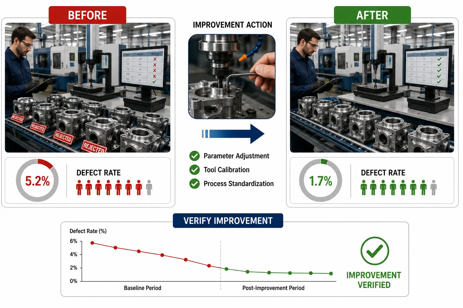
Verifying the success of a continuous improvement project is a critical stage in mechanical engineering QA/QC because implementing an improvement does not automatically demonstrate that the intended result has been achieved. A process change may appear successful immediately after implementation, yet the apparent improvement could result from temporary production conditions, reduced inspection coverage, changes in product mix, altered sampling, measurement differences or short-term variation. Professional verification therefore requires objective comparison of reliable before-and-after performance data, supported by appropriate defect percentages, process measurements, quality indicators and operational evidence.

In mechanical engineering and manufacturing environments, improvement projects may target dimensional accuracy, welding quality, machining stability, assembly reliability, inspection efficiency, material waste, cycle time, rework, rejection or equipment performance. Whatever the improvement objective, the verification process should establish a valid baseline, collect comparable post-improvement data and determine whether the observed change is statistically and operationally meaningful. The objective is not simply to demonstrate that a number has moved in the desired direction, but to determine whether the improvement is genuine, sustained, attributable to the intervention and consistent with applicable quality requirements.

For a Level 6 mechanical engineering professional, this requires analytical judgement rather than simple percentage comparison. Before-and-after data must be interpreted in context. The engineer should consider sample size, measurement methods, production conditions, specification changes, process variation, defect classification, product mix and other factors that may influence the results. A well-controlled verification process provides evidence that an improvement has delivered its intended benefit and creates a reliable basis for standardising the improved process.

Understanding improvement verification

Improvement verification is the structured process of determining whether an implemented change has achieved its defined performance objective using reliable and comparable evidence.

The basic concept can be represented as:

Baseline measurement → Improvement implementation → Post-improvement measurement → Comparison → Analysis → Verification → Standardisation

The comparison should normally address the specific problem identified at the beginning of the project.

For example, if a machining project was designed to reduce dimensional rejection from 5% to below 2%, the verification process should directly evaluate dimensional rejection before and after the intervention.

It should not rely only on unrelated measures such as production volume or machine utilisation.

Purpose of before-and-after comparison

Before-and-after comparison provides a practical method of determining whether performance has changed following an improvement.

A typical comparison may include:

  • Defect percentage.
  • Rejection percentage.
  • Rework percentage.
  • First-pass acceptance.
  • Cycle time.
  • Material waste.
  • Process variation.
  • Customer complaints.
  • Quality escapes.
  • Equipment downtime.
  • Inspection findings.

The selected measures should correspond directly to the original improvement objective.

Related definitions and key concepts

TermDefinitionMechanical engineering application
BaselineValid reference performance measured before improvementAverage rejection before process modification
Post-improvement dataPerformance information collected after implementationDefect rate following tooling change
Defect percentageProportion of inspected units containing a defined defectPercentage of components with dimensional defects
Rejection ratePercentage of inspected units rejected against requirementsRejected mechanical components
Rework ratePercentage or quantity requiring additional processingComponents requiring corrective machining
ImprovementMeasurable positive change against an established baselineReduction in dimensional defects
VerificationEvidence-based assessment confirming whether intended results were achievedComparing pre- and post-project rejection
ValidationConfirmation that a method or process is suitable for its intended purposeConfirming measurement method reliability
Performance gapDifference between actual and required performanceRejection rate above target
Control periodDefined period used to assess sustained performanceThree months after implementation
ComparabilityDegree to which two datasets can validly be comparedSame inspection method before and after
Statistical significanceEvidence that an observed difference is unlikely to be explained by random variation aloneTesting whether defect reduction is meaningful
SustainabilityAbility of an improvement to remain effective over timeStable low defect rate after implementation
StandardisationFormal adoption of a proven improved processUpdating the controlled work procedure
Control planDefined approach for maintaining process performanceOngoing monitoring after improvement

Establishing a reliable baseline

A valid baseline is one of the most important elements of improvement verification.

The baseline should represent normal process performance before the improvement is introduced.

Relevant baseline information may include:

  • Number of components produced.
  • Number of components inspected.
  • Number of defects.
  • Number of rejected components.
  • Number requiring rework.
  • Defect categories.
  • Production period.
  • Machine or workstation.
  • Product family.
  • Inspection method.
  • Applicable specification.
  • Measurement equipment.
  • Relevant environmental or operating conditions.

For example, if a machining process normally produces 1,000 components per month and 50 are rejected, the baseline rejection rate is:

This 5% value becomes the reference point for subsequent comparison.

Why baseline quality matters

Without a reliable baseline, it is difficult to establish whether improvement has actually occurred.

Consider a project that reports a post-improvement rejection rate of 2%.

The figure sounds positive, but its significance depends on the baseline.

If the baseline was:

  • 8%, the improvement is substantial.
  • 3%, the improvement is modest.
  • 1%, performance has deteriorated.

Therefore, post-improvement performance should always be interpreted against an appropriate reference.

Defining the improvement objective

Before implementation, the project should establish a measurable objective.

Examples include:

  • Reduce dimensional rejection from 5% to below 2%.
  • Reduce rework from 7% to below 3%.
  • Reduce average assembly cycle time from 55 minutes to 45 minutes.
  • Reduce material waste by 15%.
  • Increase first-pass acceptance from 91% to 97%.
  • Reduce recurring weld defects by 40%.

A clearly defined objective makes subsequent verification more straightforward.

Calculating defect percentages

Defect percentage is one of the most useful measures for verifying mechanical quality improvements.

The basic formula is:

For example:

Before improvement:

  • 80 defective components.
  • 2,000 inspected.

After improvement:

  • 30 defective components.
  • 2,000 inspected.

The defect percentage has therefore fallen from 4% to 1.5%.

Calculating percentage improvementManufacturing Defect Reduction Before and After

The relative improvement can be calculated as:

Using the previous example:

This indicates a 62.5% relative reduction in the defect rate.

The distinction between percentage-point reduction and relative percentage improvement should be maintained.

The defect rate fell by:

  • 2.5 percentage points.
  • 62.5% relative to the original defect rate.

Calculating absolute defect reduction

Another useful measure is the absolute reduction:

For the example:

This means the defect percentage reduced by 2.5 percentage points.

Comparing first-pass acceptance

First-pass acceptance can provide another perspective.

Suppose:

Before improvement:

  • First-pass acceptance = 92%.

After improvement:

  • First-pass acceptance = 97%.

The improvement is:

percentage points.

This can be particularly useful where the improvement project aims to reduce rework and improve process quality at the first inspection stage.

Comparing rework rates

Rework can consume labour, materials, machine capacity and inspection resources.

Suppose:

  • Baseline rework rate = 6%.
  • Post-improvement rework rate = 2.5%.

The reduction is:

percentage points.

Relative reduction:

This provides stronger evidence of improvement than simply stating that “rework decreased”.

Ensuring data comparability

Before-and-after data should be collected under sufficiently comparable conditions.

The engineer should examine whether there were changes in:

  • Product type.
  • Production volume.
  • Material grade.
  • Machine.
  • Tooling.
  • Inspection method.
  • Measurement equipment.
  • Sampling method.
  • Product specification.
  • Operator group.
  • Production shift.
  • Environmental conditions.
  • Production sequence.

If major differences exist, the datasets may require segmentation or qualification before direct comparison.

Example of poor comparison

Suppose a machining project reports:

Before improvement:

  • 6% defect rate on a complex component.

After improvement:

  • 2% defect rate on a simpler component.

It would be inappropriate to conclude that the process improvement reduced defects by 67% without considering the change in product complexity.

The post-improvement population is not directly comparable.

Controlling the measurement method

Measurement consistency is essential.

If the measurement system changes between baseline and post-improvement periods, the observed improvement may partly reflect measurement differences rather than genuine process improvement.

The review should therefore confirm:

  • Same measurement principle where appropriate.
  • Appropriate measurement equipment.
  • Valid calibration status.
  • Consistent units.
  • Consistent inspection criteria.
  • Consistent defect definitions.
  • Appropriate measurement resolution.

Reviewing defect definitions

Defect classification must remain consistent.

For example, if “dimensional defect” previously included all deviations greater than the specification tolerance, the same definition should normally be used after improvement.

Changing the defect definition can create an artificial improvement.

Controlling inspection coverage

Inspection coverage is another major consideration.

Suppose:

Before improvement:

  • 1,000 components inspected.
  • 50 defects found.

After improvement:

  • 1,000 components inspected.
  • 20 defects found.

The comparison is relatively straightforward.

However, if only 300 components were inspected after improvement, the lower number of defects does not necessarily demonstrate improved quality.

The engineer should compare rates and assess whether the sampling approach remains representative.

Using equivalent sample sizes

Equivalent sample sizes can simplify comparison, but identical sample sizes are not always necessary.

The important issue is that the samples should be:

  • Representative.
  • Appropriately selected.
  • Relevant to the same process.
  • Measured using comparable methods.
  • Sufficient to support the intended conclusion.

Using trend analysis

A single post-improvement measurement may not be sufficient to establish success.

A stronger approach is to monitor performance over multiple periods.

For example:

PeriodDefect Rate
Baseline5.2%
Month 13.7%
Month 22.8%
Month 32.1%
Month 41.9%
Month 51.8%

This pattern provides stronger evidence of sustained improvement than a single result of 1.8%.

Monitoring control charts after improvement

Control charts can help determine whether the improvement has stabilised the process.

For example, after a tooling improvement:

  • X-bar values remain centred.
  • R-chart variation decreases.
  • No unusual patterns appear.
  • Defect percentages decline.

This provides additional evidence that the process has improved rather than simply producing a temporary favourable result.

Distinguishing improvement from normal variation

Manufacturing processes naturally contain variation.

A small change in defect rate may occur without any intervention.

For example:

  • Month 1: 3.1%.
  • Month 2: 2.9%.
  • Month 3: 3.0%.

This may represent normal process variation rather than meaningful improvement.

The engineer should therefore examine the size, consistency and statistical behaviour of the change.

Considering statistical significance

Where appropriate, statistical methods can be used to determine whether before-and-after differences are meaningful.

The exact method depends on:

  • Type of data.
  • Sample size.
  • Distribution.
  • Measurement characteristics.
  • Comparison objective.

For defect proportions, appropriate proportion-based analysis may be considered.

For continuous measurements such as shaft diameter, methods based on means, variation or distribution may be appropriate.

Statistical testing should support engineering judgement rather than replace it.

Practical interpretation of statistical evidence

Suppose:

Before improvement:

  • 100 defects in 2,000 units.
  • Defect rate = 5%.

After improvement:

  • 92 defects in 2,000 units.
  • Defect rate = 4.6%.

The numerical reduction exists, but it may be too small to demonstrate meaningful improvement depending on process variation and statistical analysis.

By contrast:

Before:

  • 100 defects.
  • After:
  • 30 defects.

The difference is much larger and provides stronger evidence, particularly if the sampling and measurement conditions are comparable.

Assessing practical significance

Statistical significance and practical significance are not identical.

A very large production dataset may show that a tiny reduction is statistically detectable.

However, the reduction may not be operationally valuable.

Engineering teams should therefore consider:

  • Quality benefit.
  • Cost benefit.
  • Reliability benefit.
  • Customer impact.
  • Production impact.
  • Safety implications.
  • Resource requirements.

Practical example: machining defect reduction

A CNC machining cell records 4.8% dimensional rejection before improvement.

An engineering team introduces a controlled tooling-management change.

After implementation:

  • Month 1: 3.2%.
  • Month 2: 2.4%.
  • Month 3: 1.9%.
  • Month 4: 1.8%.

The target was below 2%.

The evidence suggests:

  • Rejection has decreased substantially.
  • The target has been achieved.
  • Improvement has continued across several months.
  • The result is not limited to one short production period.

The team can therefore proceed to verify process stability and standardise the successful change.

Practical example: welding defect reduction

A fabrication process records:

  • Baseline weld defect rate: 7.5%.
  • Target: below 4%.
  • Post-improvement rate: 3.6%.

However, further analysis shows that inspection coverage was reduced after the improvement.

The team should not immediately conclude that the project succeeded.

They should first determine whether:

  • Equivalent inspection coverage was maintained.
  • Defect definitions remained consistent.
  • Sampling remained representative.
  • The apparent reduction reflects genuine quality improvement.

Practical example: assembly cycle-time improvement

A mechanical assembly project aims to reduce cycle time.

Baseline:

  • Average cycle time = 62 minutes.

Post-improvement:

  • Average cycle time = 48 minutes.

However, rework also increases from 3% to 8%.

The project cannot be considered fully successful solely because cycle time improved.

The broader performance picture indicates that faster assembly may have compromised quality.

The verification should therefore consider both:

  • Cycle time.
  • Quality performance.

Balanced improvement verification

Improvement projects should be assessed against their intended objectives and potential unintended consequences.

Relevant measures may include:

  • Defect rate.
  • Rejection rate.
  • Rework.
  • Cycle time.
  • Material waste.
  • Productivity.
  • Customer complaints.
  • Equipment performance.
  • Inspection findings.

An improvement that reduces cost while increasing defects may require reassessment.

Using before-and-after comparison tables

A comparison table can communicate results clearly.

Performance MeasureBeforeAfterChangeInterpretation
Rejection rate5.0%1.8%-3.2 pointsStrong improvement
Rework rate6.0%2.1%-3.9 pointsStrong improvement
First-pass acceptance92%97%+5 pointsImproved
Cycle time52 min48 min-4 minImproved
Material waste8.5%6.4%-2.1 pointsImproved

This format allows the engineering team to assess whether the project delivered balanced improvement.

Establishing acceptance criteria for project success

Before implementation, the project should define what constitutes success.

For example:

The project will be considered successful when:

  • Dimensional rejection remains below 2%.
  • First-pass acceptance exceeds 97%.
  • Rework remains below 3%.
  • No new critical defects are introduced.
  • Performance remains stable for three consecutive months.

Defined criteria prevent subjective declarations of success.

Verifying unintended consequences

An improvement should be evaluated for secondary effects.

Potential unintended effects include:

  • Increased material consumption.
  • Reduced inspection coverage.
  • Increased equipment stress.
  • Increased operator workload.
  • New defect categories.
  • Increased maintenance requirements.
  • Increased customer complaints.

For example, reducing machining cycle time may increase tool wear.

The project should therefore evaluate both the intended benefit and possible secondary effects.

Comparing defect categories before and after

Overall defect percentage can hide shifts in defect composition.

Suppose total defects fall from 10% to 4%.

However:

  • Dimensional defects fall significantly.
  • Surface defects remain unchanged.
  • A new alignment defect appears.

The project may have achieved its primary objective but introduced a new issue.

Therefore, defect-category analysis should complement overall defect percentages.

Using Pareto analysis after improvement

Pareto analysis can identify whether the dominant defect categories have changed.

Before improvement:

  • Dimensional defects: 50%.
  • Surface defects: 25%.
  • Assembly defects: 15%.
  • Other: 10%.

After improvement:

  • Dimensional defects: 20%.
  • Surface defects: 45%.
  • Assembly defects: 25%.
  • Other: 10%.

The overall defect rate may have fallen, but surface defects have become the dominant remaining problem.

This information supports the next improvement cycle.

Verifying customer-related performance

Where the project affects customer-facing quality, verification should include:

  • Customer complaints.
  • Customer rejection.
  • Quality escapes.
  • Returned components.
  • Concession requests.
  • Customer inspection results.

Internal performance improvement should not be declared fully successful if external quality performance deteriorates.

Establishing a post-improvement monitoring period

An appropriate monitoring period should be established before final project closure.

The period depends on:

  • Production volume.
  • Failure frequency.
  • Process cycle.
  • Product risk.
  • Customer requirements.
  • Defect severity.

A high-volume process may generate sufficient evidence within weeks.

A low-volume critical component may require a much longer period.

Sustained improvement versus temporary improvement

A temporary reduction may result from:

  • Short-term operator attention.
  • Increased supervision.
  • Special inspection.
  • Reduced production volume.
  • Limited production mix.
  • Temporary equipment conditions.

Sustained improvement should continue after normal operating conditions resume.

Standardising successful improvements

Once improvement has been verified, the organisation should determine whether the change should become part of the standard process.

This may involve updating:

  • Work instructions.
  • Inspection plans.
  • Control plans.
  • Process parameters.
  • Quality procedures.
  • Training materials.
  • Maintenance schedules.
  • KPI targets.
  • Risk assessments.

Standardisation helps prevent the process from returning to its previous condition.

Improvement verification workflow

A structured verification process can follow these stages:

  1. Define the improvement objective.
  2. Establish the baseline.
  3. Validate baseline data.
  4. Implement the improvement.
  5. Define the post-improvement monitoring period.
  6. Collect comparable performance data.
  7. Verify inspection and measurement methods.
  8. Calculate defect percentages.
  9. Calculate relevant performance changes.
  10. Compare before-and-after results.
  11. Analyse trends.
  12. Review control-chart behaviour where applicable.
  13. Assess statistical significance where appropriate.
  14. Evaluate practical significance.
  15. Check for unintended consequences.
  16. Review customer-facing performance.
  17. Confirm achievement against predefined criteria.
  18. Continue monitoring for sustainability.
  19. Standardise the improvement.
  20. Document the verification outcome.

Documentation required for verification

A robust improvement project should retain evidence such as:

  • Baseline reports.
  • Post-improvement reports.
  • Inspection results.
  • Defect records.
  • Statistical calculations.
  • Control charts.
  • KPI reports.
  • Corrective-action records.
  • Process-change documentation.
  • Validation records.
  • Management review records.
  • Updated procedures.

This provides traceability and supports future improvement projects.

Common errors when verifying improvement

Comparing percentages without checking sample conditions

Different sample populations can produce misleading results.

Using only one post-improvement result

A single result may not demonstrate sustained improvement.

Ignoring measurement changes

A new inspection system may influence apparent defect rates.

Changing the defect definition

A narrower definition can create an artificial reduction.

Ignoring product mix

Different products may have different inherent defect risks.

Focusing on one KPI

An improvement in one indicator may be accompanied by deterioration elsewhere.

Declaring success too early

Short-term improvement may not represent sustainable performance.

Ignoring customer outcomes

Internal quality improvement does not automatically guarantee customer satisfaction.

Benefits of precise before-and-after verification

Effective verification provides:

  • Objective evidence of project success.
  • Clear measurement of quality improvement.
  • Better engineering decision-making.
  • Reduced reliance on assumptions.
  • Stronger corrective-action validation.
  • Improved process stability.
  • Better resource allocation.
  • Stronger customer confidence.
  • Evidence for management review.
  • Improved quality-system effectiveness.
  • Reliable lessons for future projects.
  • Stronger continual improvement.

Case Study: Verifying a machining improvement project

Background

A mechanical manufacturing organisation produces precision shafts. Inspection data shows that dimensional rejection has increased to 5.2%.

The improvement team identifies an opportunity to improve tooling control and process monitoring.

The project objective is established as:

“Reduce dimensional rejection from 5.2% to below 2% while maintaining required production output and inspection coverage.”

Baseline

Before implementation:

  • Production: 4,000 components.
  • Rejected components: 208.
  • Rejection rate: 5.2%.
  • Rework rate: 6.1%.
  • First-pass acceptance: 91.5%.

The data is validated against controlled inspection records.

Improvement implementation

The engineering team introduces a controlled process change involving:

  • Improved tooling monitoring.
  • Defined tool-life controls.
  • More structured dimensional monitoring.
  • Enhanced trend review.

Post-improvement data

After implementation:

PeriodRejectionReworkFirst-Pass Acceptance
Baseline5.2%6.1%91.5%
Month 13.6%4.2%94.0%
Month 22.7%3.1%95.6%
Month 31.9%2.4%97.0%
Month 41.7%2.1%97.4%

Analysis

The rejection rate decreased from 5.2% to 1.7%.

Absolute reduction:

percentage points.

Relative improvement:

The result therefore represents approximately a 67.3% relative reduction in rejection rate.

The improvement also appears sustained across four months.

Verification

The predefined objective was below 2%.

The process achieved:

  • 1.9% in Month 3.
  • 1.7% in Month 4.

The first-pass acceptance rate also improved.

Importantly, the team verifies that:

  • Inspection coverage remained consistent.
  • Product mix remained comparable.
  • Measurement methods remained controlled.
  • No new major defect category emerged.
  • Production output remained acceptable.

The evidence therefore supports the conclusion that the improvement project achieved its intended quality objective.

Standardisation

Following verification, the organisation updates:

  • Tool-management procedures.
  • Inspection controls.
  • Process monitoring requirements.
  • Relevant work instructions.
  • KPI reporting.
  • Training material.

The improved process becomes part of normal production control.

Using verification results for continual improvement

Verification should not be considered the final activity in the quality cycle. The results should provide information for future improvement.

If the project achieves its target, the organisation can:

  • Standardise the improvement.
  • Identify additional improvement opportunities.
  • Update the baseline.
  • Establish a new performance target.
  • Monitor long-term stability.

If the project fails to achieve its target, the team should:

  • Review the original problem definition.
  • Reassess the root-cause analysis.
  • Examine implementation effectiveness.
  • Review measurement reliability.
  • Identify additional contributing factors.
  • Develop a revised intervention.

This creates a continual improvement cycle rather than a one-time project.

Conclusion

Verifying the success of a continuous improvement project requires more than demonstrating that a performance indicator has changed. A professional QA/QC verification process establishes a reliable baseline, collects comparable post-improvement data, calculates precise defect percentages, analyses trends and evaluates whether the observed change is meaningful and sustained. Mechanical engineering teams should consider rejection, rework, first-pass acceptance, dimensional conformity, cycle time, material waste and other relevant indicators according to the original improvement objective.

The most reliable verification combines quantitative before-and-after comparison with engineering judgement. Data must be validated, inspection coverage must remain appropriate, measurement methods must be comparable and changes in product mix or specifications must be considered. Where appropriate, statistical analysis and control charts can provide additional evidence that the improvement represents a genuine change rather than normal process variation.

A successful improvement should also be evaluated for unintended consequences and monitored over an appropriate period before the change is fully standardised. Once evidence confirms that the desired performance has been achieved and sustained, the improved method can be incorporated into controlled procedures, inspection plans, KPIs and work instructions. This evidence-based approach strengthens mechanical QA/QC systems, improves process reliability, reduces defects and rework, supports customer confidence and provides a measurable foundation for continual improvement across engineering and manufacturing operations.

3 Present actionable quality data summaries and statistical findings to technical teams to guide collaborative root-cause investigations

Effective mechanical engineering quality management depends not only on collecting accurate data, but also on communicating that information in a form that technical teams can understand, challenge, interpret and use. Quality data has limited practical value when it remains buried within inspection records, spreadsheets, test reports or statistical software. The engineering professional must therefore convert complex inspection and production information into concise, accurate and actionable summaries that clearly identify the performance issue, quantify its significance and provide a reliable starting point for collaborative root-cause investigation.

In mechanical manufacturing and QA/QC environments, technical teams may include mechanical engineers, production engineers, quality engineers, inspectors, maintenance personnel, welding specialists, manufacturing supervisors and other relevant technical personnel. Each group may interpret the same quality information from a different operational perspective. A dimensional trend may indicate potential machining instability to a manufacturing engineer, possible tooling deterioration to a production specialist, or a measurement-system concern to a QA/QC engineer. Effective presentation therefore requires both technical accuracy and contextual clarity. The objective is not to dictate the root cause prematurely, but to present evidence that allows the team to investigate possible causes systematically.

Actionable quality data summaries should connect the measured problem with its operational significance. Rather than presenting hundreds of raw measurements, the QA/QC professional should identify meaningful patterns, defect frequencies, process trends, control-chart signals, KPI changes, Pareto distributions and relevant statistical findings. The summary should make clear what has changed, where the change is concentrated, how reliable the evidence is and what questions require further investigation. This creates a collaborative evidence-based environment in which root-cause analysis is guided by facts rather than assumptions, personal opinions or isolated observations.

Understanding actionable quality data summaries

An actionable quality data summary is a concise presentation of validated quality information that enables a technical team to understand a performance issue and determine appropriate investigative actions.

It should normally communicate:

  • The problem being investigated.
  • The affected process or component.
  • The relevant time period.
  • Current performance.
  • Historical or target performance.
  • Defect frequency.
  • Significant trends.
  • Statistical findings.
  • Areas requiring investigation.
  • Data limitations.
  • Recommended investigation priorities.

The summary should answer a practical question:

“What does the available evidence tell the technical team, and what should they investigate next?”

Difference between raw data and actionable information

Raw data consists of individual observations.

For example:

  • Shaft 001: 50.03 mm.
  • Shaft 002: 50.05 mm.
  • Shaft 003: 50.08 mm.
  • Shaft 004: 50.11 mm.
  • Shaft 005: 50.14 mm.

This information may be useful, but it does not immediately communicate the broader process condition.

An actionable summary could state:

“Measured shaft diameter has shown a progressive upward trend during the current production run, with recent observations approaching the upper acceptance boundary. The trend should be investigated for potential process drift, tooling condition or measurement-related factors.”

The second presentation converts individual measurements into information that supports engineering investigation.

Purpose of presenting statistical findings

Statistical findings provide an objective basis for understanding variation and performance.

Relevant findings may include:

  • Mean.
  • Median.
  • Range.
  • Standard deviation.
  • Defect percentage.
  • Rejection rate.
  • Process capability indicators.
  • Control-chart signals.
  • Trend direction.
  • Frequency distributions.
  • Pareto results.
  • Before-and-after comparisons.
  • Correlation patterns where technically appropriate.

The purpose is not to overwhelm technical teams with statistical calculations. Statistical information should be selected according to the engineering decision it supports.

Key concepts and definitions

ConceptDefinitionApplication in mechanical QA/QC
Quality data summaryConcise presentation of relevant quality informationWeekly dimensional defect report
Actionable dataInformation that supports a specific decision or investigationIdentifying a machine with increasing rejection
Statistical findingResult obtained through appropriate statistical analysisSustained process shift
Root-cause investigationStructured investigation to identify underlying causesInvestigating repeated machining defects
BaselineReference performance used for comparisonHistorical defect rate
TrendPattern of change over timeIncreasing vibration readings
VariationDifference between process observationsShaft diameter spread
OutlierObservation substantially different from the main datasetAbnormal pressure measurement
Defect ratePercentage of defective itemsWeld defect percentage
Rejection ratePercentage of items rejectedFinal inspection rejection
Pareto analysisMethod for ranking problems by frequency or impactIdentifying dominant defect categories
Control chartStatistical tool for monitoring process behaviourX-bar and R chart monitoring
MeanArithmetic average of observationsAverage component diameter
RangeDifference between highest and lowest valueWithin-subgroup dimensional spread
Standard deviationMeasure of data dispersion around the meanVariation in measured dimensions
Process shiftSustained change in process levelChanged machining dimension average
EvidenceVerified information supporting an assessmentControlled inspection records
Data limitationFactor affecting interpretation or confidenceSmall sample size
Investigation priorityIssue selected for further technical analysisHighest-frequency defect category
Root-cause hypothesisPotential explanation requiring investigationPossible tool wear

Principles of effective quality data presentation

A professional summary should be:

  • Accurate.
  • Concise.
  • Relevant.
  • Traceable.
  • Objective.
  • Visually clear.
  • Statistically appropriate.
  • Technically understandable.
  • Free from unsupported conclusions.
  • Linked to an investigation objective.

The summary should distinguish between what the data demonstrates and what the team suspects.

Presenting facts separately from hypotheses

This is particularly important during root-cause investigation.

For example:

Fact:

“Dimensional rejection increased from 2.1% to 5.4% over six weeks.”

Possible hypothesis:

“Tool wear may be contributing to the dimensional drift.”

The second statement should not be presented as established fact unless investigation confirms it.

This distinction prevents the team from becoming anchored to an unverified explanation.

Establishing the investigation context

Before presenting detailed statistics, the QA/QC professional should briefly explain the context.

The summary should identify:

  • Product or component.
  • Manufacturing process.
  • Relevant machine or workstation.
  • Quality characteristic.
  • Applicable acceptance criterion.
  • Time period.
  • Performance concern.

For example:

“The review concerns the dimensional conformity of 50 mm bearing seats produced on Machining Cell 3 during the previous six-week production period.”

This gives the technical team a clear frame of reference.

Presenting baseline performance

The baseline should normally be shown before the current condition.

For example:

  • Historical rejection rate: 1.8%.
  • Current rejection rate: 4.7%.
  • Target: below 2%.

The data immediately establishes a performance gap.

Presenting trends rather than isolated values

Quality Data to Root Cause Investigation

A trend can be more informative than a single measurement.

For example:

WeekRejection Rate
11.7%
22.0%
32.4%
43.1%
53.8%
64.7%

The pattern suggests progressive deterioration.

The technical team can then investigate possible changes during the same period.

Connecting trends with operational events

Trend information becomes more useful when aligned with known process events.

Relevant events may include:

  • Tool changes.
  • Machine maintenance.
  • Material changes.
  • Process-parameter changes.
  • Operator changes.
  • Equipment relocation.
  • Software updates.
  • Fixture replacement.
  • Supplier changes.
  • Production-rate changes.

For example, if dimensional rejection begins increasing immediately after a tooling change, the event becomes a relevant investigation point.

It is not automatically the root cause.

Presenting control-chart findings

Control charts provide useful evidence about process behaviour.

A quality summary might report:

“Seven consecutive subgroup averages have remained above the established centre line, indicating a potential process shift requiring investigation.”

This is more useful than simply showing the chart without interpretation.

The summary should explain:

  • What the chart monitors.
  • What unusual pattern has been observed.
  • Whether the condition is isolated or sustained.
  • What process area should be investigated.

X-bar and R chart findings

For processes monitored using X-bar and R charts, the summary may distinguish:

X-bar findings:

  • Shift in process average.
  • Sustained run.
  • Trend.
  • Points outside control limits.

R-chart findings:

  • Increasing variation.
  • Unusual range.
  • Reduced or unstable within-subgroup variation.

For example:

“The X-bar chart indicates a progressive upward shift in average shaft diameter, while the R chart remains comparatively stable. Investigation should therefore consider factors affecting process centring rather than assuming a major increase in short-term variation.”

This type of statement provides useful technical direction without declaring a cause.

Presenting Pareto findings

Pareto analysis is particularly useful when numerous defect categories exist.

Suppose a production department records:

  • Dimensional defects: 38%.
  • Weld porosity: 27%.
  • Surface damage: 15%.
  • Alignment defects: 11%.
  • Other: 9%.

The summary might state:

“Dimensional defects and weld porosity account for 65% of recorded quality failures and should receive priority during the initial root-cause investigation.”

This helps the team focus resources on the most significant contributors.

Using defect percentages

Defect percentages allow teams to compare performance across different production volumes.

For example:

  • Batch A: 20 defects from 1,000 components = 2%.
  • Batch B: 40 defects from 4,000 components = 1%.

Although Batch B has twice as many defective components numerically, its defect rate is lower.

This demonstrates why raw defect counts alone can be misleading.

Presenting process capability findings

Where appropriate, process capability analysis can help establish whether a process is capable of consistently meeting specified requirements.

The summary should explain the practical meaning of the result rather than simply presenting a numerical index.

For example:

“The process capability assessment indicates insufficient margin between observed process variation and the specified tolerance. Further investigation of process centring and variation is recommended.”

The technical team can then examine:

  • Process centring.
  • Variation.
  • Measurement reliability.
  • Machine condition.
  • Tooling.
  • Process parameters.

Presenting measurement uncertainty

Quality summaries should acknowledge measurement limitations where relevant.

For example:

“Observed dimensional differences are relatively small compared with the measurement system resolution; therefore, measurement-system capability should be confirmed before attributing the difference to process deterioration.”

This prevents technical teams from acting on potentially insignificant differences.

Identifying outliers

An outlier is an observation that differs substantially from the main pattern.

For example, pressure measurements may be:

  • 98 bar.
  • 99 bar.
  • 100 bar.
  • 101 bar.
  • 118 bar.

The 118 bar value requires investigation.

However, it should not automatically be deleted.

Possible explanations include:

  • Genuine process event.
  • Measurement error.
  • Instrument problem.
  • Data-entry error.
  • Temporary operating condition.

The summary should identify the outlier and recommend appropriate verification.

Avoiding automatic deletion of outliers

Removing unusual data simply because it weakens the analysis can create misleading conclusions.

The engineer should establish:

  • Whether the value is valid.
  • Whether the measurement was correctly recorded.
  • Whether the instrument was functioning correctly.
  • Whether the process was genuinely different at that time.

Only justified data treatment should be applied.

Using statistical summaries appropriately

Different datasets require different summaries.

For continuous dimensional data, useful measures may include:

  • Mean.
  • Standard deviation.
  • Range.
  • Minimum.
  • Maximum.
  • Distribution.

For categorical defect data:

  • Frequency.
  • Percentage.
  • Pareto ranking.

For time-based performance:

  • Trend.
  • Moving average where appropriate.
  • Control-chart behaviour.

The method should reflect the type of information being analysed.

Data visualisation for technical teams

Good visualisation can improve technical understanding.

Useful formats include:

  • Control charts.
  • Trend graphs.
  • Pareto charts.
  • Histograms.
  • Scatter plots.
  • Before-and-after comparisons.
  • KPI dashboards.
  • Process maps.

Visuals should be:

  • Clearly labelled.
  • Properly scaled.
  • Easy to interpret.
  • Linked to the engineering issue.
  • Free from unnecessary decoration.

Avoiding overcrowded dashboards

A dashboard containing dozens of graphs may make critical information harder to identify.

A technical summary should prioritise:

  • The most important performance indicator.
  • The key trend.
  • The dominant defect.
  • The relevant statistical signal.
  • The immediate investigation question.

Additional data can remain available as supporting evidence.

Presenting data in layers

A useful approach is to present information in three levels.

Level 1: Executive summary

  • Problem.
  • Magnitude.
  • Trend.
  • Priority.

Level 2: Technical evidence

  • Charts.
  • Defect percentages.
  • Statistical results.
  • Process comparisons.

Level 3: Supporting data

  • Detailed inspection records.
  • Raw measurements.
  • Batch information.
  • Equipment records.

This allows different technical audiences to access the appropriate level of detail.

Connecting data with root-cause investigation

A quality summary should lead naturally into investigation.

For example:

“Dimensional rejection has increased from 2.0% to 5.1% over six weeks. Seventy percent of defects originate from Machining Cell 2, and the increase began shortly after a tooling change. The team should investigate tooling condition, process centring, measurement records and relevant maintenance history.”

This is actionable because it identifies:

  • What changed.
  • Where.
  • By how much.
  • When.
  • Potential investigation areas.

It does not state that the tooling change caused the problem without evidence.

Structured root-cause investigation questions

The summary can support questions such as:

  • What changed when the problem began?
  • Which machine is most affected?
  • Which defect category dominates?
  • Is the problem associated with a particular material batch?
  • Is the process average shifting?
  • Is process variation increasing?
  • Has tooling condition changed?
  • Has maintenance history changed?
  • Is the measurement system reliable?
  • Is the problem limited to one shift?
  • Are similar components affected?
  • Has the customer requirement changed?

Cross-functional interpretation

Different technical disciplines may provide different interpretations.

For example:

Quality engineer:

“Inspection data shows increasing dimensional rejection.”

Manufacturing engineer:

“The trend coincides with a change in tooling.”

Maintenance engineer:

“Machine spindle vibration increased during the same period.”

Production supervisor:

“The process began running at a higher output rate.”

The combined evidence may reveal an interaction that would not have been identified by one discipline alone.

Practical example: machining defect investigation

A machining operation reports increasing diameter defects.

The QA/QC team prepares the following summary:

  • Historical rejection: 1.9%.
  • Current rejection: 4.8%.
  • 74% of defects are diameter-related.
  • 69% originate from Machine 4.
  • X-bar data shows an upward process shift.
  • R-chart variation remains broadly stable.
  • The trend began shortly after a tooling change.

The technical team now has a focused investigation.

Possible investigation areas include:

  • Tool condition.
  • Tool offset.
  • Machine alignment.
  • Process parameters.
  • Measurement system.
  • Material condition.

The summary does not claim the tool is defective.

Practical example: welding quality

A fabrication department records 420 weld-related defects during a quarter.

Pareto analysis shows:

  • Porosity: 42%.
  • Incomplete fusion: 26%.
  • Undercut: 18%.
  • Other: 14%.

The summary should focus initial investigation on porosity and incomplete fusion because together they represent 68% of recorded weld defects.

Additional data may then be presented concerning:

  • Welding stations.
  • Material batches.
  • Production shifts.
  • Inspection results.
  • Relevant process records.

Practical example: bearing assembly

A bearing assembly line reports increasing rework.

The summary shows:

  • Baseline rework: 2.8%.
  • Current rework: 6.4%.
  • Alignment defects: 61% of rework.
  • 75% of alignment defects originate from one workstation.
  • The workstation changed fixtures four weeks earlier.

The technical team should investigate:

  • Fixture condition.
  • Fixture alignment.
  • Assembly sequence.
  • Component positioning.
  • Measurement method.

Again, the fixture change is a relevant investigation factor, not an automatically confirmed root cause.

Practical example: pressure-testing data

A pressure-testing process produces:

  • Historical average: 100 bar.
  • Current average: 96 bar.
  • Increasing variation.
  • Three recent results below the defined acceptance condition.

The summary should clearly distinguish:

  • Average shift.
  • Variation change.
  • Specification requirements.
  • Number of affected units.

The technical team can then investigate:

  • Test equipment.
  • Pressure source.
  • Component condition.
  • Test procedure.
  • Environmental factors.

Using statistical evidence responsibly

Statistical results should be presented with sufficient context.

A statement such as:

“Standard deviation increased by 40%”

is incomplete without identifying:

  • The measurement.
  • The period.
  • The baseline.
  • The sample size.
  • The significance of the change.

A stronger statement is:

“Standard deviation for shaft diameter increased from 0.018 mm to 0.025 mm across comparable production samples, indicating increased dimensional dispersion that warrants investigation.”

Explaining confidence and limitations

Technical teams should know when evidence is strong and when it is uncertain.

Relevant limitations may include:

  • Small sample size.
  • Missing records.
  • Inconsistent measurement methods.
  • Product-mix differences.
  • Limited historical data.
  • Changed specifications.
  • Incomplete maintenance information.

A transparent statement might be:

“The observed trend is consistent across three production batches; however, the available data does not yet establish whether the change is statistically significant.”

This is more professionally defensible than presenting uncertainty as certainty.

Data summary structure

A practical quality data summary can follow this structure:

Problem

State the issue clearly.

Evidence

Present the most important measurements.

Trend

Show how performance has changed.

Comparison

Compare current performance with baseline or target.

Statistical finding

Explain relevant statistical evidence.

Concentration

Identify the machine, product, defect or process area most affected.

Investigation focus

Identify the technical questions that require further analysis.

Limitations

State important data-quality constraints.

Recommended technical presentation sequence

A technical review can follow this sequence:

  1. State the problem.
  2. Present the baseline.
  3. Present current performance.
  4. Show the trend.
  5. Identify the dominant defect.
  6. Present statistical findings.
  7. Identify affected process areas.
  8. Highlight relevant process changes.
  9. Explain data limitations.
  10. Define investigation questions.
  11. Agree investigation responsibilities.
  12. Establish follow-up actions.

Benefits of actionable quality summaries

Effective data presentation supports:

  • Faster problem recognition.
  • Better root-cause analysis.
  • Cross-functional collaboration.
  • Reduced reliance on assumptions.
  • More efficient engineering meetings.
  • Better prioritisation.
  • Improved corrective actions.
  • Stronger evidence-based decisions.
  • Better management visibility.
  • Improved quality performance.
  • Reduced recurring defects.
  • More effective continual improvement.

Common mistakes to avoid

Presenting too much raw data

Large tables can hide important trends.

Presenting statistics without interpretation

Numbers alone may not explain their operational significance.

Declaring a root cause prematurely

A correlation or timing relationship does not automatically prove causation.

Ignoring data limitations

Uncertainty should be communicated openly.

Using misleading graphs

Poor scales or inappropriate chart types can distort interpretation.

Focusing only on averages

Variation and distribution may be equally important.

Ignoring operational context

Statistical results should be considered alongside engineering events.

Failing to identify an action

A quality summary should help the team determine what needs investigation next.

Case Study: Presenting quality data to a cross-functional engineering team

Background

A mechanical manufacturing facility produces precision housings. Final inspection reports indicate an increase in bore-diameter rejection.

The QA/QC department collects six weeks of data.

Findings

The analysis identifies:

  • Historical rejection rate: 1.6%.
  • Current rejection rate: 4.5%.
  • Bore-diameter defects: 72% of all rejected components.
  • Machine B: 67% of bore-related defects.
  • X-bar chart: progressive upward movement.
  • R chart: relatively stable variation.
  • Tool change: implemented near the beginning of the trend.
  • Measurement equipment: calibration remains current.

Quality data summary

The QA/QC engineer presents:

“Bore-diameter rejection has increased from 1.6% to 4.5% during the previous six-week period. Bore-related defects represent 72% of all rejections, with 67% occurring on Machine B. X-bar results indicate a progressive shift in the process average while within-subgroup variation remains comparatively stable. The trend began shortly after a tooling change. The measurement equipment remains within its current calibration status.”

Investigation questions

The team agrees to investigate:

  • Tool condition.
  • Tool offset.
  • Machine alignment.
  • Tool-change procedure.
  • Process parameters.
  • Fixture condition.
  • Material variation.

Cross-functional contributions

The manufacturing engineer reviews tooling.

The maintenance engineer reviews machine condition.

The quality engineer verifies measurement data.

The production supervisor reviews process changes.

The combined approach allows the team to examine multiple potential contributors without prematurely assigning blame.

Outcome

Further investigation confirms that tool wear and an inadequate tool-life threshold contributed to the dimensional drift.

The organisation implements:

  • Improved tool-life monitoring.
  • Revised tool-change criteria.
  • Additional process monitoring.

Subsequent data shows the rejection rate falling below the established target.

The case demonstrates how a concise statistical summary can provide the foundation for collaborative technical investigation.

Quality data presentation workflow

A robust workflow can be summarised as:

Data collection → Data validation → Statistical analysis → Pattern identification → Summary preparation → Technical presentation → Collaborative investigation → Root-cause analysis → Corrective action → Verification

Each stage should maintain traceability to the original evidence.

Preparing the data

Before analysis:

  • Confirm data sources.
  • Remove duplicate records where justified.
  • Correct verified data-entry errors.
  • Confirm measurement units.
  • Confirm specification revision.
  • Check missing information.
  • Identify unusual observations.
  • Confirm inspection method.

Selecting the most relevant statistics

Not every statistical calculation is required.

Select measures that answer the investigation question.

For dimensional variation:

  • Mean.
  • Range.
  • Standard deviation.
  • Control-chart behaviour.

For defect categories:

  • Frequency.
  • Percentage.
  • Pareto ranking.

For time-related performance:

  • Trend.
  • Average.
  • Variation.
  • Period comparison.

Translating statistics into engineering language

Statistical terminology should be connected to practical implications.

Instead of:

“The mean shifted by 0.08 mm.”

Use:

“The average shaft diameter has shifted upward by 0.08 mm, reducing the available margin to the upper acceptance boundary.”

This allows the technical team to understand why the statistical finding matters.

Maintaining objectivity

The presentation should avoid emotionally loaded statements.

Prefer:

“Defect frequency increased by 38%.”

Rather than:

“The production team performed poorly.”

Prefer:

“Machine B accounts for 67% of the recorded bore-diameter defects.”

Rather than:

“Machine B is causing the problem.”

The first statements are evidence-based.

Closing the technical review

At the end of the presentation, the team should have:

  • A shared understanding of the problem.
  • Agreed evidence.
  • Defined investigation boundaries.
  • Identified potential contributing factors.
  • Assigned investigation responsibilities.
  • Established follow-up requirements.

This transforms quality reporting into an active engineering improvement process.

Conclusion

Presenting actionable quality data summaries and statistical findings is a critical capability in mechanical engineering QA/QC because effective root-cause investigation depends on reliable evidence and shared technical understanding. Raw inspection records, defect logs and production measurements become significantly more valuable when they are converted into concise summaries showing the performance baseline, current condition, trends, defect concentrations and relevant statistical signals. The objective is to give technical teams enough accurate information to ask the right questions without prematurely deciding what the root cause must be.

A professional quality data presentation should distinguish facts from hypotheses, acknowledge limitations and connect statistical findings with the physical manufacturing process. Control charts, Pareto analysis, defect percentages, trend analysis, process capability information and KPI comparisons can reveal where problems are concentrated and how performance is changing. When these findings are presented clearly to quality, production, maintenance and engineering personnel, each discipline can contribute its own technical knowledge to the investigation.

The strongest approach is therefore collaborative and evidence-driven. The QA/QC professional provides verified information, explains its significance and identifies investigation priorities, while the wider technical team examines possible contributing factors and develops appropriate root-cause hypotheses. This process supports more effective corrective actions, reduces recurring mechanical defects, strengthens process control and creates a reliable foundation for continual improvement.