
Lesson 4: Use data-driven strategies to improve process efficiency and component reliability.
Modern mechanical engineering and manufacturing environments increasingly depend on accurate data to improve process efficiency, product quality, equipment reliability, and operational performance. Data-driven strategies enable engineering and QA/QC professionals to move beyond reactive problem-solving by using inspection results, production records, process measurements, equipment condition data, defect trends, maintenance histories, and statistical evidence to identify opportunities for improvement. In mechanical manufacturing, effective data analysis can reveal process bottlenecks, recurring component defects, equipment deterioration, excessive variation, inefficient operating conditions, and emerging reliability risks. This creates a stronger foundation for evidence-based engineering decisions and continuous improvement.
This lesson examines how mechanical engineering data can be transformed into practical improvement strategies that enhance manufacturing consistency and component reliability. It explores the relationship between process performance, statistical evidence, quality indicators, equipment condition, and engineering interventions. Attention is given to analysing performance trends, identifying the causes of inefficiency, evaluating component reliability, prioritising improvement opportunities, and selecting corrective or preventive actions based on measurable evidence. By applying structured data analysis, engineers can determine whether improvements should focus on process parameters, tooling, equipment condition, inspection frequency, maintenance practices, material control, production methods, or other relevant operational factors. The approach supports more effective quality assurance and quality control while reducing unnecessary waste, rework, downtime, scrap, and premature component failure.
From an international mechanical engineering and QA/QC perspective, data-driven improvement also supports measurable performance management and long-term operational reliability. Well-structured engineering data provides traceable evidence for evaluating whether corrective actions have delivered sustainable results rather than temporary improvements. Historical inspection records, statistical process indicators, reliability measures, maintenance information, and production performance data can be compared before and after an intervention to determine its effectiveness. This lesson therefore develops a systematic approach to using engineering evidence for process optimisation, defect reduction, reliability improvement, and informed decision-making. The principles are relevant to mechanical manufacturing, fabrication, maintenance, industrial production, precision engineering, plant operations, and quality management environments where consistent performance and reliable components are essential.
1: Design Action Plans That Use Historical Quality Data to Optimise Machining Feeds, Speeds, or Welding Parameters for Better Production Output
Data-driven process optimisation is a fundamental component of modern mechanical engineering, manufacturing quality assurance, quality control and production management. In machining and welding operations, process parameters directly influence productivity, dimensional accuracy, surface quality, weld integrity, tool life, energy consumption, material utilisation and overall production efficiency. Selecting feeds, speeds or welding parameters solely through experience or trial and error can produce inconsistent results, particularly when materials, machines, tooling, joint configurations or production conditions change. Historical quality data provides a stronger evidence base because it allows engineers to understand how previous parameter settings affected measurable production outcomes.
An effective action plan therefore connects historical inspection results with the operating conditions that produced those results. Instead of simply asking whether a component passed or failed inspection, the engineering team examines why a particular process produced the observed result and whether a different parameter combination could improve productivity without compromising quality. This approach supports evidence-based optimisation, where production output is improved while dimensional tolerances, surface condition, weld quality, structural integrity and process stability remain within specified requirements.
The objective is not to maximise machining speed or welding productivity in isolation. A technically sound action plan must balance productivity, quality, equipment capability, tool or consumable life, safety, energy use, material behaviour and repeatability. A parameter change that increases output but produces excessive tool wear, distortion, porosity, dimensional variation or rework is not a genuine improvement. Sustainable optimisation requires the relationship between process parameters and quality performance to be demonstrated through reliable data, controlled trials and subsequent verification.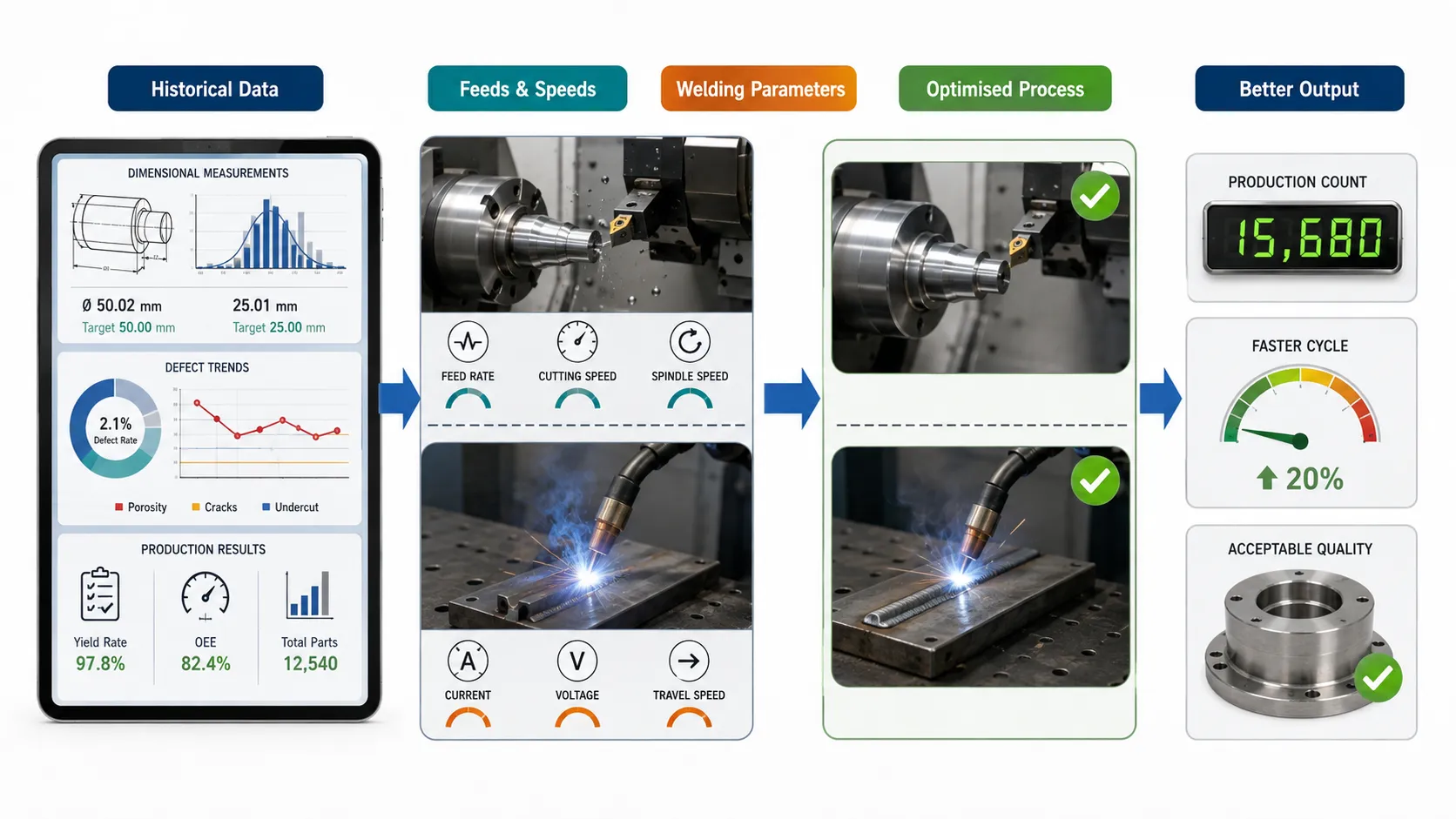
Understanding Data-Driven Process Optimisation
Data-driven process optimisation is the structured use of historical and current engineering information to identify improved operating conditions and implement controlled changes to a manufacturing process.
In mechanical production, relevant information may include:
- Historical dimensional inspection results.
- Surface-finish measurements.
- Weld inspection results.
- Non-destructive testing results.
- Tool-life records.
- Cutting speeds.
- Feed rates.
- Depth of cut.
- Spindle speed.
- Welding current.
- Welding voltage.
- Travel speed.
- Heat input.
- Interpass temperature.
- Material grades.
- Material thickness.
- Defect frequency.
- Rework levels.
- Scrap rates.
- Production cycle times.
- Machine downtime.
- Maintenance records.
- Operator observations.
- Environmental conditions.
When these variables are analysed together, relationships between process settings and quality outcomes can be identified.
Key Definitions and Concepts
| Term | Definition | Application in Mechanical Engineering |
|---|---|---|
| Historical Quality Data | Previously recorded information about process and product quality | Dimensional results from previous machining batches |
| Action Plan | Structured sequence of activities designed to achieve a defined improvement | Controlled optimisation of machining parameters |
| Feed Rate | Rate at which cutting tool or workpiece advances through the material | Influences productivity, cutting forces and surface quality |
| Cutting Speed | Relative speed between cutting edge and workpiece surface | Influences material removal rate and tool wear |
| Spindle Speed | Rotational speed of a machine spindle | Used to establish appropriate machining conditions |
| Depth of Cut | Thickness of material removed during a machining pass | Influences cutting forces and productivity |
| Welding Current | Electrical current used during welding | Influences arc characteristics and heat input |
| Welding Voltage | Electrical potential used during welding | Affects arc behaviour and weld characteristics |
| Travel Speed | Rate at which the welding torch or electrode moves along the joint | Influences heat input and weld profile |
| Heat Input | Thermal energy introduced into the weld per unit length | Important for weld quality and distortion control |
| Process Optimisation | Systematic improvement of process conditions | Improving output while maintaining conformity |
| Process Capability | Ability of a stable process to produce results within specified limits | Evaluating dimensional consistency |
| Baseline | Established reference level for process performance | Current production cycle time before optimisation |
| Defect Rate | Proportion of production containing identified defects | Measuring quality before and after parameter changes |
| Cycle Time | Time required to complete a defined production operation | Used to evaluate productivity improvement |
| Tool Life | Period during which a tool performs acceptably | Comparing different cutting conditions |
| Rework | Additional processing required to correct a non-conforming product | Indicator of process inefficiency |
| Scrap | Material or product rejected as unsuitable for intended use | Important cost and quality indicator |
| Validation | Evidence-based confirmation that a process or change achieves its intended outcome | Confirming a new parameter set |
| Optimisation | Selection of the most effective operating conditions within defined constraints | Balancing quality, output and equipment performance |
Why Historical Quality Data Matters
Historical data allows engineering teams to move from assumptions towards measurable evidence. A production record might show that a machining operation previously required 12 minutes per component. Inspection records may show that the process consistently achieved dimensional conformity but generated occasional surface-finish problems.
Further analysis may reveal that:
- The machine was operating at a conservative cutting speed.
- Tool wear was relatively low.
- Cycle time was longer than necessary.
- Surface-finish defects occurred mainly near the end of tool life.
- Certain material batches produced higher cutting resistance.
- Increasing feed rate under controlled conditions could potentially reduce cycle time.
The engineering response should therefore not simply increase feed rate. Instead, historical evidence should be used to design a controlled optimisation programme.
Establishing a Reliable Data Foundation
Before designing an action plan, the quality of historical data must be assessed.
Engineers should confirm:
- Measurement units are consistent.
- Equipment identification is recorded.
- Tool identification is available where relevant.
- Material grades are traceable.
- Process parameters are recorded accurately.
- Inspection methods are consistent.
- Measurement equipment was suitably calibrated.
- Defects are classified consistently.
- Production conditions are comparable.
- Maintenance interventions are documented.
Poor historical data can result in incorrect conclusions.
Connecting Process Parameters With Quality Outcomes
The central principle is to establish relationships between what the process did and what the inspection system observed.
For machining, the analysis may connect:
Machining parameters → Cutting behaviour → Tool condition → Component quality → Production output
For welding, the relationship may be:
Welding parameters → Heat input and arc behaviour → Weld characteristics → Inspection results → Production performance
This approach allows the engineer to identify parameter combinations associated with acceptable and unacceptable outcomes.
Designing a Data-Driven Action Plan
A professional action plan should begin with a clearly defined improvement objective.
Examples include:
- Reduce machining cycle time by a defined percentage.
- Increase production output while maintaining dimensional conformity.
- Reduce tool-related defects.
- Reduce weld repair rates.
- Improve weld consistency.
- Reduce excessive heat input.
- Increase tool life.
- Reduce surface-finish variation.
- Reduce component rejection.
- Improve overall process stability.
The objective should be measurable.
For example:
“Reduce average machining cycle time while maintaining all specified dimensional and surface-quality requirements.”
is stronger than:
“Make the machining process faster.”
Step 1: Establish the Current Baseline
The existing process must be documented before changes are introduced.
A baseline may include:
- Current feed rate.
- Current cutting speed.
- Current spindle speed.
- Current depth of cut.
- Average cycle time.
- Tool life.
- Dimensional capability.
- Surface-finish performance.
- Defect rate.
- Scrap rate.
- Rework rate.
- Machine utilisation.
For welding, the baseline may include:
- Current current range.
- Voltage.
- Travel speed.
- Welding position.
- Electrode or consumable type.
- Heat input.
- Preheat requirements.
- Interpass temperature.
- Weld inspection results.
- Repair rate.
- Production time.
Step 2: Identify Historical Performance Patterns
Historical data should be examined for relationships.
For example, an engineer may discover that:
- Higher cutting speed reduced cycle time.
- Excessive speed increased tool wear.
- Higher feed rates increased productivity.
- Excessive feed rates increased surface roughness.
- Lower welding travel speed increased heat input.
- Excessive heat input increased distortion.
- Increased welding current improved penetration within a controlled range.
- Excessive current increased undesirable weld characteristics.
These patterns provide starting points for optimisation.
Step 3: Segment the Data
Historical data should not always be analysed as one combined dataset.
Useful categories may include:
- Material grade.
- Component size.
- Machine.
- Tool type.
- Welding process.
- Joint configuration.
- Operator group.
- Production line.
- Production period.
- Tool condition.
- Batch.
- Equipment condition.
Segmentation prevents unrelated conditions from being mixed together.
Step 4: Identify the Critical Process Variables
Not every recorded variable has equal importance.
For machining, critical variables may include:
- Cutting speed.
- Feed rate.
- Depth of cut.
- Tool geometry.
- Tool material.
- Coolant condition.
- Workpiece material.
- Machine rigidity.
For welding:
- Current.
- Voltage.
- Travel speed.
- Heat input.
- Consumable type.
- Joint preparation.
- Preheat.
- Interpass temperature.
- Welding position.
The engineer should identify which variables have the strongest relationship with the targeted quality or productivity outcome.
Step 5: Analyse the Quality Consequences
Parameter changes should always be assessed against quality performance.
For machining, consider:
- Dimensional accuracy.
- Surface roughness.
- Burr formation.
- Tool wear.
- Chatter.
- Cutting forces.
- Thermal effects.
For welding, consider:
- Weld profile.
- Penetration.
- Fusion.
- Porosity.
- Cracking.
- Distortion.
- Heat-affected-zone effects.
- Inspection results.
The objective is to identify the acceptable operating window rather than a single parameter that maximises production speed.
Step 6: Develop an Operating Window
A useful action plan establishes:
- Lower operating boundary.
- Target operating condition.
- Upper operating boundary.
- Monitoring requirements.
- Quality acceptance criteria.
- Intervention conditions.
This creates a controlled operating window.
For example:
| Process Variable | Lower Condition | Target Condition | Upper Condition | Main Monitoring Point |
|---|---|---|---|---|
| Cutting speed | Conservative | Optimised | Maximum validated | Tool wear |
| Feed rate | Low | Optimised | Maximum validated | Surface finish |
| Depth of cut | Light | Balanced | Maximum validated | Cutting force |
| Welding current | Lower validated range | Target | Upper validated range | Weld quality |
| Travel speed | Slow validated range | Target | Fast validated range | Heat input |
| Cycle time | Existing baseline | Reduced target | — | Production output |
The values used in an actual workplace must come from the applicable machine capability, material requirements, approved procedures, engineering specifications and validated process conditions.
Machining Feed Optimisation
Feed rate strongly influences material removal and production time.
Increasing feed rate can potentially:
- Reduce machining time.
- Increase material removal rate.
- Improve production throughput.
However, excessive feed can also increase:
- Cutting forces.
- Tool wear.
- Surface roughness.
- Burr formation.
- Dimensional instability.
- Machine vibration.
Therefore, historical inspection data should be examined to determine the point at which productivity gains begin to compromise quality.
Cutting Speed Optimisation
Cutting speed influences:
- Cutting temperature.
- Tool wear.
- Productivity.
- Surface condition.
- Material removal behaviour.
Historical tool-life records can show how different speeds affected tool longevity.
An action plan should therefore compare:
Cutting speed → Cycle time → Tool life → Defect rate → Cost per component.
A faster process is not necessarily economically superior if tool consumption and rejection increase significantly.
Depth-of-Cut Optimisation
Depth of cut can influence production efficiency because larger cuts may reduce the number of machining passes.
However, higher depth of cut can increase:
- Cutting force.
- Machine loading.
- Tool stress.
- Deflection.
- Thermal effects.
Historical machine and inspection records can help identify suitable conditions.
Welding Parameter Optimisation
Welding parameters must be considered as an interacting system rather than isolated values.
For example:
Current + voltage + travel speed → Heat input → Weld behaviour → Inspection outcome
Increasing one parameter without considering the others can change the overall process.
Historical weld inspection records can help determine which parameter combinations previously produced stable results.
Heat Input Considerations
Heat input is an important variable in many welding applications.
Changes in heat input can influence:
- Weld penetration.
- Weld profile.
- Distortion.
- Cooling behaviour.
- Heat-affected-zone characteristics.
- Productivity.
The action plan should therefore use historical welding data to understand how changes affected inspection outcomes.
Using Statistical Evidence
Data-driven optimisation should use appropriate statistical techniques where sufficient data exists.
Useful techniques include:
- Mean comparison.
- Range analysis.
- Standard deviation.
- Trend analysis.
- Control charts.
- Pareto analysis.
- Regression analysis.
- Correlation analysis.
- Process capability analysis.
- Before-and-after comparison.
Statistical evidence should support engineering judgement rather than replace it.
Before-and-After Analysis
A simple optimisation study may compare:
Before intervention:
- Cycle time: 12 minutes.
- Defect rate: 3%.
- Tool life: 800 components.
After controlled optimisation:
- Cycle time: 10 minutes.
- Defect rate: 2%.
- Tool life: 850 components.
This would suggest improvement, provided the data is statistically and operationally comparable.
Practical Example: CNC Turning
A production line manufactures precision shafts.
Historical data shows:
- Average cycle time: 10.5 minutes.
- Stable dimensions at the existing parameter setting.
- Tool replacement approximately every 900 components.
- Surface-finish defects increase near the end of tool life.
The production team wants higher output.
The QA/QC engineer reviews historical records and identifies a parameter range that previously produced shorter cycle times without significant dimensional deterioration.
A controlled trial is designed.
The trial includes:
- Defined parameter changes.
- Limited production quantity.
- Increased dimensional inspection.
- Surface-finish checks.
- Tool-condition monitoring.
- Defect recording.
The results show reduced cycle time while maintaining acceptable quality.
The change can then move into controlled implementation following appropriate technical validation and approval.
Practical Example: Welding Production
A fabrication facility experiences inconsistent weld production times.
Historical records show that operators use slightly different travel speeds within the permitted process conditions.
Inspection records show that slower travel speeds are associated with higher heat input and increased distortion in certain joint configurations.
The engineering team develops an action plan based on:
- Historical weld inspection results.
- Travel-speed records.
- Heat-input calculations.
- Distortion measurements.
- Repair records.
A controlled operating range is established and validated.
The result is improved consistency without simply increasing welding speed indiscriminately.
Practical Example: Tool Wear
A machining operation has acceptable dimensional quality for most of the tool’s life.
Historical records show that dimensional variation begins increasing after approximately 1,000 cycles.
Rather than waiting for components to become non-conforming, the action plan introduces:
- Increased inspection frequency after a defined cycle count.
- Tool-condition checks.
- Historical trend comparison.
- Planned replacement criteria.
This converts historical inspection data into a preventive quality strategy.
Balancing Productivity and Reliability
A major engineering consideration is the relationship between output and equipment reliability.
An aggressive process may produce:
- Higher output.
- Higher tool wear.
- More machine stress.
- Greater maintenance requirements.
- Increased quality variation.
A conservative process may produce:
- Lower tool wear.
- Stable quality.
- Lower output.
- Longer cycle times.
The objective is to identify the best overall operating condition rather than simply selecting the fastest setting.
Key Performance Indicators
An action plan should identify measurable indicators.
Potential KPIs include:
- Cycle time.
- Production output.
- First-pass yield.
- Defect rate.
- Scrap rate.
- Rework rate.
- Tool life.
- Machine utilisation.
- Downtime.
- Surface-finish compliance.
- Dimensional capability.
- Weld repair rate.
- Inspection failure rate.
- Cost per component.
Risk Assessment Before Implementation
Before changing process parameters, the engineering team should consider:
- Equipment capability.
- Material behaviour.
- Tool capacity.
- Component criticality.
- Safety implications.
- Quality requirements.
- Existing approved procedures.
- Potential failure mechanisms.
- Inspection requirements.
Higher-risk parameter changes require stronger validation and control.
Controlled Trials
A controlled trial should define:
Objective
What improvement is being tested?
Variables
Which process parameter will change?
Constraints
Which parameters must remain controlled?
Sample
How many components or welds will be evaluated?
Measurements
What quality and performance characteristics will be measured?
Acceptance Criteria
What results are required for approval?
Decision
What evidence will determine whether the change is adopted?
Monitoring During the Trial
During a trial, engineers should monitor:
- Dimensional results.
- Surface quality.
- Tool condition.
- Weld inspection results.
- Machine behaviour.
- Production time.
- Defect frequency.
- Operator observations.
Any unexpected deterioration should trigger investigation.
Verification of Results
The improvement must be verified using objective evidence.
Questions should include:
- Did cycle time decrease?
- Did production output increase?
- Did quality remain acceptable?
- Did tool life improve or deteriorate?
- Did defects increase?
- Did rework change?
- Did machine loading change?
- Did the improvement remain stable?
Standardising Successful Improvements
Once a process change has been validated, the organisation should update appropriate controlled information.
This may include:
- Process instructions.
- Parameter sheets.
- Inspection plans.
- Control plans.
- Maintenance requirements.
- Training information.
- Quality records.
- Process monitoring requirements.
This ensures that the improvement becomes part of controlled production practice.
Managing Failed Trials
Not every optimisation trial will succeed.
A trial may fail because:
- Productivity improves but quality deteriorates.
- Tool wear becomes excessive.
- Weld distortion increases.
- Machine vibration increases.
- Dimensional variation becomes unstable.
- The expected relationship does not appear.
Failed trials should still be documented because they provide engineering knowledge.
Common Mistakes in Data-Driven Optimisation
Changing Too Many Variables at Once
If feed rate, speed and depth of cut are changed simultaneously, it may become difficult to identify which change caused the result.
Focusing Only on Production Speed
Higher output does not represent improvement if defect and rework rates increase.
Ignoring Tool Condition
Historical parameter performance can change as tools deteriorate.
Mixing Different Materials
Different material grades may respond differently to the same process conditions.
Ignoring Machine Condition
A parameter that worked on a well-maintained machine may not produce the same result on deteriorated equipment.
Using Insufficient Data
A small dataset may not represent normal process behaviour.
Ignoring Measurement Uncertainty
Apparent improvement may result from measurement variation rather than actual process improvement.
Implementing Changes Without Verification
A promising trial result does not automatically demonstrate long-term stability.
Key Benefits of Data-Driven Action Plans
Improved Production Output
Optimised process conditions can reduce unnecessary cycle time.
Better Quality Consistency
Historical evidence helps identify parameter ranges associated with stable quality.
Reduced Scrap
Early identification of inefficient process conditions can reduce non-conforming production.
Reduced Rework
Stable parameters can reduce repeated correction activities.
Improved Tool Utilisation
Tool-life data supports more informed replacement decisions.
Better Equipment Performance
Controlled operating conditions can reduce unnecessary machine stress.
Improved Decision-Making
Engineering decisions are supported by measurable evidence.
Greater Process Stability
Validated operating windows can reduce uncontrolled parameter variation.
Stronger Continuous Improvement
Each completed optimisation cycle creates additional historical knowledge.
Professional Data-Driven Action Plan Structure
A robust action plan can use the following structure:
1. Define the Problem
Clearly describe the existing inefficiency or reliability issue.
2. Establish the Baseline
Record current performance.
3. Collect Historical Evidence
Review relevant quality and production records.
4. Identify Influential Variables
Determine which parameters may affect performance.
5. Analyse Relationships
Compare process settings with quality outcomes.
6. Establish Improvement Targets
Define measurable objectives.
7. Conduct Risk Assessment
Identify potential negative consequences.
8. Design Controlled Trials
Change parameters within appropriate technical limits.
9. Measure Results
Collect quality and productivity evidence.
10. Analyse Results
Compare the trial against the baseline.
11. Validate the Improvement
Confirm that the change is stable and acceptable.
12. Standardise
Update controlled process information where required.
13. Monitor
Continue collecting data to confirm long-term performance.
Case Study: Data-Driven Machining Optimisation
Background
A precision engineering company manufactures mechanical shafts using CNC turning equipment. Production management identifies cycle time as an improvement opportunity, but quality records show that dimensional defects increase when tooling approaches the end of its useful life.
Historical Analysis
The engineering team examines twelve months of records.
The analysis identifies:
- Cycle times for each batch.
- Feed and speed settings.
- Tool identification.
- Tool-change intervals.
- Dimensional inspection results.
- Surface-finish results.
- Rework levels.
- Material batch information.
A pattern emerges showing that certain operating conditions provide shorter cycle times without significant deterioration in dimensional quality.
Action Plan
The team establishes:
- A baseline process.
- A controlled parameter range.
- Increased inspection during the trial.
- Tool-condition monitoring.
- Defined acceptance criteria.
- A post-trial review.
Trial
A limited production batch is manufactured under the revised conditions.
Measurements are collected at predetermined intervals.
Results
The revised condition produces:
- Reduced cycle time.
- Stable dimensional results.
- Acceptable surface finish.
- No significant increase in tool-related defects.
Verification
The process is monitored over subsequent production batches.
The improvement remains stable.
Engineering Outcome
The revised parameter condition is adopted through the organisation’s controlled process-management system.
This example demonstrates that optimisation is not simply about selecting a faster machining setting. It involves historical analysis, risk assessment, controlled experimentation, quality verification and sustained monitoring.
Case Study: Welding Parameter Improvement
Background
A fabrication operation experiences inconsistent weld production times and variable distortion.
Historical inspection records are reviewed alongside welding parameter data.
Findings
The analysis identifies differences in:
- Travel speed.
- Welding current.
- Voltage.
- Heat input.
- Joint configuration.
Higher heat input is associated with increased distortion in a specific production configuration.
Action
The engineering team develops a controlled parameter range and introduces additional monitoring of:
- Weld dimensions.
- Distortion.
- Inspection results.
- Production time.
- Repair frequency.
Outcome
The revised process provides improved production consistency while maintaining the required weld quality.
The organisation then updates controlled production documentation and continues monitoring.
Conclusion
Designing action plans from historical quality data enables mechanical engineering organisations to improve production output without treating productivity and quality as separate objectives. Machining feeds, cutting speeds, spindle speeds, depths of cut and welding parameters can have significant effects on cycle time, tool life, heat input, dimensional stability, surface quality, weld integrity and equipment performance. Historical inspection and production records provide valuable evidence for understanding these relationships and identifying operating conditions that have previously produced reliable results.
A professional data-driven action plan begins with a clearly defined improvement objective and a reliable baseline. Historical data is then validated, segmented and analysed to identify relationships between process parameters and measurable outcomes. The engineer should consider material characteristics, machine condition, tooling, inspection methods and production conditions before drawing conclusions. Statistical methods such as trend analysis, correlation, regression, process capability analysis and before-and-after comparisons can strengthen the evidence base, while engineering judgement remains essential for interpreting the physical meaning of the results.
Process optimisation should always be controlled. Increasing feed rate, cutting speed, welding current or other parameters simply because they appear to increase output can create unacceptable consequences such as accelerated tool wear, dimensional drift, surface defects, excessive heat input, distortion, equipment stress or increased rework. The appropriate objective is therefore to establish a validated operating window in which production efficiency is improved while component quality, process stability and mechanical reliability remain within specified requirements.
Controlled trials provide an effective bridge between historical evidence and full-scale implementation. Each trial should have a defined objective, controlled variables, measurable acceptance criteria and appropriate inspection requirements. Results should be compared with the baseline to determine whether the change genuinely improves performance. Where an improvement is validated, relevant process instructions, inspection plans, parameter sheets and monitoring arrangements should be updated through appropriate document-control processes.
The long-term value of this approach is that every improvement activity contributes to the organisation’s engineering knowledge base. Historical quality data becomes progressively more useful as it accumulates information about tool life, process capability, material behaviour, defect mechanisms, equipment performance and parameter sensitivity. This supports continuous improvement, reduces waste and rework, strengthens QA/QC decision-making, improves production efficiency and contributes to more reliable mechanical components and manufacturing processes.
2: Develop Component Reliability Strategies, Such as Mean Time Between Failures (MTBF) Targets, Based on Real-World Asset Breakdown Data
Component reliability is a fundamental consideration in mechanical engineering, manufacturing, maintenance, QA/QC and asset performance management. A component may satisfy its dimensional and material requirements when manufactured, yet its long-term value depends on how consistently it performs under actual operating conditions. Reliability strategies therefore need to connect design expectations and quality requirements with evidence from real equipment breakdowns, maintenance records, inspection findings and operational histories.
Mean Time Between Failures (MTBF) is one of the useful reliability indicators for analysing repairable mechanical assets. When calculated correctly, MTBF can help an engineering team understand how frequently equipment or components experience functional failures during defined operating periods. However, MTBF should not be treated simply as a target number. A meaningful reliability strategy examines why failures occur, under what conditions they occur, whether the failures are recurring, how severe their consequences are, and whether corrective actions produce measurable improvement.
Using real-world asset breakdown data makes reliability planning more evidence-based. Historical breakdown records can reveal recurring bearing failures, seal deterioration, shaft damage, coupling problems, gearbox faults, lubrication-related failures, overheating, misalignment and other mechanical conditions. When these records are systematically classified and analysed, the organisation can establish realistic reliability targets and develop strategies for reducing failure frequency, improving component life and increasing operational availability.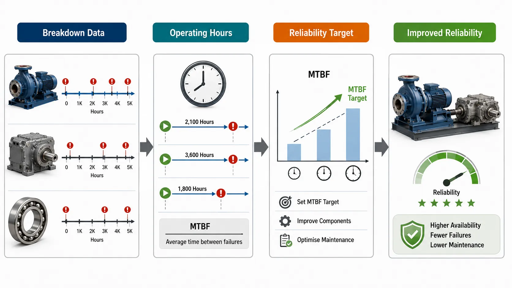
Understanding Component Reliability
Reliability refers to the ability of a component, machine or system to perform its required function for a specified period under stated operating conditions.
In mechanical engineering, reliability is influenced by:
- Component design.
- Material selection.
- Manufacturing quality.
- Installation quality.
- Operating conditions.
- Loading.
- Lubrication.
- Alignment.
- Environmental conditions.
- Maintenance practices.
- Inspection effectiveness.
- Component age.
- Failure mechanisms.
Reliability is therefore not controlled by manufacturing quality alone. A high-quality component can still experience premature failure if it is incorrectly installed, overloaded, poorly lubricated or operated outside its intended conditions.
Key Definitions and Concepts
| Term | Definition | Mechanical Engineering Application |
|---|---|---|
| Reliability | Probability that an asset performs its required function for a specified period under stated conditions | Reliability of a gearbox during continuous operation |
| MTBF | Mean operating time between failures of a repairable asset or component | Average operating hours between pump failures |
| Failure | Loss of the ability to perform a required function | Bearing can no longer operate within required conditions |
| Breakdown | An event where equipment becomes unavailable or unable to perform its intended function | Pump stops unexpectedly during production |
| Failure Rate | Frequency at which failures occur within a defined operating population or period | Bearing failures per operating hour |
| Availability | Proportion of required time that equipment is capable of operating | Production equipment available during scheduled hours |
| Maintainability | Ease and speed with which an asset can be restored after failure | Time required to replace a failed bearing |
| MTTF | Mean Time To Failure, commonly used for non-repairable items | Average operating life of a disposable component |
| MTTR | Mean Time To Repair or restore equipment | Average time required to restore a pump |
| Preventive Maintenance | Planned maintenance performed before failure | Scheduled bearing inspection |
| Predictive Maintenance | Maintenance based on condition or predicted deterioration | Replacing a bearing based on vibration trends |
| Corrective Maintenance | Action taken to restore or improve equipment following an identified issue | Replacing a damaged coupling |
| Failure Mode | Specific manner in which a component fails | Bearing seizure |
| Root Cause | Fundamental reason a failure occurred | Lubrication failure causing bearing overheating |
| Failure Distribution | Statistical description of failures over time | Distribution of gearbox failures by operating hours |
| Reliability Target | Defined performance objective for asset reliability | Increasing MTBF from 4,000 to 5,000 hours |
| Operating Time | Time during which an asset is functioning or available for its intended operation | Pump operating hours between failures |
| Failure History | Recorded information about previous failures | Five years of bearing breakdown records |
| Critical Asset | Asset whose failure has significant safety, production or financial consequences | Main process compressor |
| Reliability Improvement | Action designed to reduce failure frequency or extend useful life | Improving lubrication control |
What MTBF Means
For a repairable asset, MTBF is generally calculated as:
MTBF = Total relevant operating time ÷ Number of relevant failures
For example, if a group of identical pumps operates for a combined 24,000 hours and experiences 6 relevant failures:
MTBF = 24,000 ÷ 6
MTBF = 4,000 operating hours per failure.
This means that, over the observed population and period, the average operating time between recorded failures was 4,000 hours.
It does not mean that every pump will operate exactly 4,000 hours before failing.
Why MTBF Must Be Interpreted Carefully
MTBF is an average.
Individual components may fail:
- Much earlier than the average.
- Close to the average.
- Much later than the average.
Therefore, MTBF should be combined with:
- Failure mode analysis.
- Failure-rate trends.
- Operating conditions.
- Component criticality.
- Maintenance history.
- Inspection results.
- Reliability distribution.
- Availability.
- Repair time.
Using MTBF alone can lead to poor engineering decisions.
Real-World Breakdown Data as a Reliability Resource
Breakdown records can provide information about:
- Failure date.
- Operating hours.
- Equipment identification.
- Component identification.
- Failure mode.
- Failure location.
- Failure severity.
- Operating conditions.
- Maintenance history.
- Repair activity.
- Replacement parts.
- Root cause.
- Downtime.
- Production impact.
The quality of the reliability strategy depends heavily on the quality and consistency of these records.
Establishing a Reliable Failure Database
Before setting MTBF targets, the organisation should establish a structured failure database.
Important fields include:
- Asset ID.
- Component ID.
- Equipment type.
- Manufacturer.
- Installation date.
- Operating hours.
- Failure date.
- Failure mode.
- Failure cause.
- Operating conditions.
- Maintenance activity.
- Repair duration.
- Replacement component.
- Production downtime.
- Corrective action.
- Verification result.
This creates traceability between equipment history and reliability performance.
Classifying Failures
Failures should be classified consistently.
Possible categories include:
Mechanical Failure
Examples:
- Shaft fracture.
- Bearing seizure.
- Gear tooth damage.
- Coupling failure.
Lubrication Failure
Examples:
- Insufficient lubrication.
- Incorrect lubricant.
- Contamination.
- Lubricant degradation.
Alignment Failure
Examples:
- Shaft misalignment.
- Coupling misalignment.
- Excessive mechanical movement.
Thermal Failure
Examples:
- Overheating.
- Excessive friction.
- Cooling-system deterioration.
Manufacturing-Related Failure
Examples:
- Dimensional defect.
- Material defect.
- Incorrect heat treatment.
- Surface defect.
Consistent classification makes trend analysis more meaningful.
Calculating MTBF From Breakdown Data
Suppose four identical mechanical pumps provide the following operating records:
- Pump A: 6,000 hours, 2 failures.
- Pump B: 5,000 hours, 1 failure.
- Pump C: 7,000 hours, 2 failures.
- Pump D: 6,000 hours, 1 failure.
Total operating time:
6,000 + 5,000 + 7,000 + 6,000 = 24,000 hours.
Total failures:
2 + 1 + 2 + 1 = 6.
Therefore:
MTBF = 24,000 ÷ 6 = 4,000 hours.
This provides a historical reliability baseline.
Developing an MTBF Target
An MTBF target should be based on evidence rather than arbitrary ambition.
The engineering team may consider:
- Current MTBF.
- Historical trend.
- Component design life.
- Operating conditions.
- Failure consequences.
- Maintenance capability.
- Supplier information.
- Improvement opportunities.
- Cost of intervention.
- Production requirements.
For example:
Current MTBF = 4,000 hours.
If historical improvement programmes have demonstrated achievable gains, an initial target might be set above the current baseline, such as:
Target MTBF = 4,500 hours.
The target should be technically justified and periodically reviewed.
Baseline Versus Target
A useful reliability strategy distinguishes between:
Baseline
What the asset currently achieves.
Target
What the organisation aims to achieve.
Threshold
The level at which intervention or escalation becomes necessary.
For example:
- Baseline MTBF: 4,000 hours.
- Improvement target: 4,500 hours.
- Minimum acceptable level: 3,800 hours.
The actual values must be established from the asset’s technical, operational and risk context.
Setting Realistic Reliability Targets
Targets should be:
- Measurable.
- Evidence-based.
- Relevant.
- Time-bound.
- Technically achievable.
- Linked to defined assets.
- Supported by reliable data.
A target such as “eliminate all failures” is generally unrealistic.
A stronger target might be:
“Increase average MTBF for the identified pump population by 15% over the next defined operating period while maintaining required safety and performance conditions.”
Failure Trend Analysis
Historical breakdown data should be plotted over time.
The analysis may identify:
- Increasing failure frequency.
- Stable failure frequency.
- Decreasing failures.
- Seasonal patterns.
- Failure clustering.
- Age-related deterioration.
A rising failure frequency may indicate deterioration or an ineffective maintenance strategy.
Failure Mode Analysis
MTBF alone does not explain why an asset fails.
Consider a pump population with:
- Bearing failures.
- Seal failures.
- Coupling failures.
The overall MTBF may look acceptable, but if bearing failures represent most breakdowns, improvement should focus on bearing-related causes.
This is why MTBF should be combined with failure-mode analysis.
Practical Reliability Strategy
A structured strategy may follow this sequence:
Historical breakdown data
↓
Data validation
↓
Failure classification
↓
Operating-time calculation
↓
MTBF baseline
↓
Failure-mode analysis
↓
Criticality assessment
↓
Root-cause investigation
↓
Improvement actions
↓
Reliability target
↓
Monitoring
↓
Verification
↓
Target review
Asset Criticality
Not every component requires the same reliability strategy.
Criticality can consider:
- Safety impact.
- Environmental impact.
- Production impact.
- Financial impact.
- Repair complexity.
- Availability of spare parts.
- Failure detectability.
A critical production compressor may require more rigorous reliability management than a non-critical auxiliary fan.
Safety-Critical Reliability
For safety-critical equipment, reliability targets must not be considered solely from a production perspective.
The strategy should incorporate:
- Applicable safety requirements.
- Functional requirements.
- Inspection requirements.
- Failure consequences.
- Redundancy where applicable.
- Proof-testing or condition-monitoring arrangements where appropriate.
Reliability improvement should never compromise safety controls.
MTBF and Availability
MTBF should be distinguished from availability.
A system may have a reasonable MTBF but poor availability if repairs take a long time.
Availability is influenced by:
- Failure frequency.
- Repair duration.
- Spare-part availability.
- Maintenance response.
- Access to skilled personnel.
Therefore, reliability strategies should often monitor MTBF together with MTTR.
MTTR and Reliability Strategy
Mean Time To Repair measures how long it takes to restore an asset following a repairable failure.
For example:
If four repairs require:
- 2 hours.
- 3 hours.
- 4 hours.
- 3 hours.
MTTR = 12 ÷ 4 = 3 hours.
An organisation can improve availability through:
- Higher MTBF.
- Lower MTTR.
- Or both.
Reliability and Maintainability
A reliable component fails less frequently.
A maintainable component can be restored efficiently when failure occurs.
An effective strategy therefore asks two questions:
- How can failure frequency be reduced?
- How can restoration time be reduced?
Identifying Recurring Failures
Historical data may show that the same component repeatedly fails.
For example:
- Bearing replaced in January.
- Bearing replaced in April.
- Bearing replaced in July.
- Bearing replaced in October.
This recurring pattern requires investigation.
Simply replacing the bearing each time may treat the symptom rather than the underlying cause.
Root-Cause Investigation
Potential causes may include:
- Misalignment.
- Overloading.
- Poor lubrication.
- Contamination.
- Incorrect installation.
- Excessive vibration.
- Incorrect component selection.
- Manufacturing defects.
The objective is to identify the mechanism that produces the recurring failure.
Reliability-Centred Thinking
Reliability improvement should focus on the function of the asset and the consequences of losing that function.
Questions include:
- What function must the component perform?
- What constitutes functional failure?
- How can failure occur?
- What are the consequences?
- Can deterioration be detected early?
- What maintenance strategy is appropriate?
- What design improvement could reduce recurrence?
Preventive Maintenance Based on MTBF
Historical MTBF data can support maintenance planning.
For example, if a component historically develops problems around a particular operating period, inspections may be scheduled before that period.
However, fixed replacement based solely on average MTBF can be inefficient.
The actual failure distribution should be considered.
Predictive Maintenance
Condition-monitoring information can strengthen reliability strategies.
Useful indicators include:
- Vibration.
- Temperature.
- Lubricant condition.
- Acoustic signals.
- Alignment.
- Wear measurements.
- Electrical or mechanical performance indicators.
When deterioration can be detected before functional failure, maintenance can be planned more effectively.
Reliability Improvement Through Condition Monitoring
Suppose historical data shows that bearing failures are often preceded by increasing vibration.
The reliability strategy can introduce:
- Regular vibration monitoring.
- Defined trend thresholds.
- Increased monitoring frequency when deterioration begins.
- Planned bearing inspection.
- Root-cause investigation.
This can reduce unexpected breakdowns.
Using Historical Data to Set Inspection Frequency
Inspection frequency should reflect:
- Failure history.
- Asset criticality.
- Rate of deterioration.
- Consequences of failure.
- Detectability.
- Operating conditions.
A component with rapidly changing condition indicators may require more frequent inspection than a stable component.
Practical Example: Pump Reliability
A plant operates ten process pumps.
Historical data shows:
- 50,000 total operating hours.
- 10 relevant failures.
MTBF:
50,000 ÷ 10 = 5,000 hours.
Further analysis shows that 60% of failures involve bearings.
The engineering team investigates:
- Lubrication practices.
- Alignment.
- Operating load.
- Bearing installation.
- Vibration.
The data indicates that several failures are associated with poor alignment.
The reliability strategy therefore focuses on:
- Improved alignment verification.
- Post-maintenance checks.
- Vibration monitoring.
- Installation controls.
- Technician training.
The MTBF target is then reviewed after the intervention.
Practical Example: Gearbox Reliability
Historical records show repeated gearbox failures.
The data reveals:
- Failures occur predominantly under high-load operation.
- Several failures involve gear tooth damage.
- Lubricant contamination is frequently recorded.
The engineering team develops a strategy involving:
- Improved lubricant cleanliness control.
- Condition monitoring.
- Load monitoring.
- Gear inspection.
- Improved maintenance intervals.
The target is not simply to replace gearboxes less frequently. The objective is to address the factors contributing to failure.
Practical Example: Bearing Population
A production line uses 100 identical bearings.
Historical records show a combined operating time of 200,000 hours and 20 relevant failures.
MTBF:
200,000 ÷ 20 = 10,000 hours.
The engineering team identifies that failures are concentrated in one operating area with higher temperature.
The reliability strategy should therefore consider environmental and operating differences rather than applying one identical intervention across all bearings.
Reliability Target Escalation
Reliability performance can be managed using defined escalation levels.
For example:
Level 1
Performance meets or exceeds target.
Action:
- Continue normal monitoring.
Level 2
Performance approaches minimum acceptable level.
Action:
- Review trends.
- Increase monitoring.
Level 3
Performance falls below the defined threshold.
Action:
- Conduct engineering investigation.
- Develop corrective action.
Level 4
Repeated critical failures occur.
Action:
- Consider design modification, replacement strategy or major intervention.
Measuring Reliability Improvement
After implementing an improvement, the organisation should calculate the new performance.
Suppose:
Before improvement:
MTBF = 4,000 hours.
After improvement:
MTBF = 4,800 hours.
Improvement:
800 hours.
Percentage improvement:
(800 ÷ 4,000) × 100 = 20%.
This provides a measurable indication of improvement.
Reliability Data Segmentation
MTBF should sometimes be calculated separately for:
- Equipment type.
- Component type.
- Manufacturer.
- Production line.
- Operating environment.
- Load category.
- Age group.
- Maintenance strategy.
This can reveal differences hidden within an overall average.
Avoiding Misleading MTBF Calculations
Engineers should avoid:
- Mixing unrelated component types.
- Counting minor events as major failures without a defined rule.
- Ignoring operating time.
- Using incomplete failure records.
- Counting planned maintenance as random failure.
- Changing failure definitions during the analysis.
- Comparing assets with significantly different operating conditions.
Consistency is essential.
Defining What Counts as a Failure
The organisation should establish clear failure criteria.
A failure might mean:
- Loss of required function.
- Performance below an approved limit.
- Safety-critical malfunction.
- Unplanned component replacement.
- Inability to meet required output.
Minor maintenance activities may not necessarily constitute failures for MTBF purposes.
The definition must be consistent throughout the dataset.
Failure Data Quality
Reliability analysis should verify:
- Accurate failure dates.
- Correct operating hours.
- Correct equipment identification.
- Correct component identification.
- Correct failure classification.
- Accurate repair records.
- Consistent failure definitions.
Poor records can produce misleading reliability targets.
Key Benefits of MTBF-Based Reliability Strategies
Evidence-Based Target Setting
Targets are linked to actual asset performance.
Reduced Unplanned Downtime
Recurring failure mechanisms can be addressed.
Improved Maintenance Planning
Maintenance resources can be allocated based on evidence.
Better Component Selection
Failure histories can support engineering decisions about component types.
Reduced Maintenance Costs
Preventing recurring failures can reduce emergency repairs.
Improved Production Availability
Higher reliability can increase operational continuity.
Better Quality Feedback
Manufacturing defects and reliability failures can be connected.
Improved Risk Management
Critical failure patterns can be identified earlier.
Stronger Continuous Improvement
Each failure contributes information for future improvement.
Common Mistakes
Treating MTBF as a Guaranteed Life
MTBF is an average, not a guarantee.
Setting Unrealistic Targets
Targets should reflect actual operating conditions and improvement potential.
Ignoring Failure Mode
A single MTBF value does not explain why failures occur.
Mixing Different Assets
Unrelated equipment should not be combined without justification.
Ignoring Operating Conditions
Load, temperature and environment influence reliability.
Counting Every Maintenance Event as Failure
Failure definitions must be established consistently.
Focusing Only on MTBF
Availability and MTTR may also be important.
Failing to Verify Improvements
A reliability intervention must be assessed using subsequent data.
Building a Reliability Dashboard
A useful reliability dashboard may include:
- Current MTBF.
- Target MTBF.
- Previous-period MTBF.
- Failure count.
- Failure rate.
- MTTR.
- Availability.
- Top failure modes.
- Critical asset status.
- Recurring failures.
- Corrective-action status.
This provides management and engineering teams with a common view of reliability performance.
Reliability Improvement Action Plan
A practical action plan may contain:
Objective
Increase reliability of a defined asset population.
Baseline
Current MTBF and failure history.
Target
Evidence-based future MTBF.
Main Failure Modes
Highest-impact recurring failures.
Root Causes
Confirmed or suspected causes requiring investigation.
Actions
Engineering, maintenance, inspection or operational improvements.
Owner
Responsible technical function.
Timescale
Defined implementation period.
Measurement
MTBF, MTTR, availability and failure frequency.
Verification
Post-implementation performance review.
Case Study: Developing an MTBF Strategy for Industrial Pumps
Background
An industrial facility operates a population of centrifugal process pumps.
Unexpected pump failures have caused production interruptions.
Historical Data
Three years of records are reviewed.
The database contains:
- Operating hours.
- Failure dates.
- Bearing replacements.
- Seal failures.
- Coupling failures.
- Maintenance activities.
- Vibration records.
- Repair durations.
Baseline Calculation
The combined operating time is 120,000 hours.
There are 24 relevant failures.
MTBF:
120,000 ÷ 24 = 5,000 hours.
Failure Analysis
The data shows:
- 12 bearing failures.
- 7 seal failures.
- 3 coupling failures.
- 2 other mechanical failures.
Bearing failures are therefore the dominant category.
Further Investigation
The engineering team reviews:
- Alignment records.
- Lubrication records.
- Operating temperature.
- Vibration trends.
- Installation practices.
A recurring relationship between poor alignment and elevated vibration is identified.
Reliability Strategy
The organisation introduces:
- Improved alignment verification.
- Post-maintenance vibration checks.
- More consistent lubrication controls.
- Increased monitoring of high-risk pumps.
- Root-cause review of recurring bearing failures.
Reliability Target
An improvement target is established above the 5,000-hour baseline based on the organisation’s technical assessment and achievable improvement potential.
Verification
Subsequent operating data is reviewed.
If failures decrease and MTBF increases sustainably, the strategy demonstrates effectiveness.
Case Study: Component Reliability in Manufacturing
A manufacturing plant experiences repeated premature failure of drive couplings.
Historical records show:
- High failure frequency on one production line.
- Increased vibration before several failures.
- Higher failure frequency following certain maintenance activities.
- Inconsistent alignment records.
The QA/QC and maintenance teams analyse the data together.
The reliability strategy introduces:
- Alignment verification.
- Installation controls.
- Vibration trend monitoring.
- Defined inspection intervals.
- Component condition records.
The organisation then monitors whether coupling failures decline and MTBF improves.
Linking Reliability With Quality Assurance
Reliability data can reveal manufacturing-quality problems.
For example, repeated failures may be associated with:
- Incorrect dimensions.
- Improper heat treatment.
- Surface defects.
- Material inconsistencies.
- Incorrect assembly.
- Welding defects.
Therefore, reliability analysis should feed information back into QA/QC systems.
Linking Reliability With Manufacturing Data
A useful reliability strategy can connect:
Manufacturing data
→ Inspection results
→ Component installation
→ Operating performance
→ Failure history
→ Root-cause analysis
→ Reliability improvement.
This creates a closed feedback loop.
Long-Term Reliability Management
Reliability strategies should not be treated as one-time projects.
The organisation should periodically review:
- MTBF trends.
- Failure patterns.
- Maintenance effectiveness.
- Asset criticality.
- Component performance.
- Supplier performance.
- Operating conditions.
- Improvement results.
Targets may need adjustment when conditions change.
Professional Principles for Reliability Strategy Development
A competent engineering approach should:
- Use verified historical breakdown data.
- Define failure consistently.
- Calculate operating time accurately.
- Treat MTBF as an average rather than a guarantee.
- Analyse failure modes.
- Consider asset criticality.
- Identify root causes.
- Set realistic reliability targets.
- Monitor MTTR and availability where appropriate.
- Verify improvement through subsequent operating data.
- Maintain traceability.
- Integrate reliability information with QA/QC and maintenance systems.
Conclusion
Developing component reliability strategies from real-world asset breakdown data enables mechanical engineering organisations to move from reactive failure response towards evidence-based reliability management. Historical breakdown records provide valuable information about how frequently components fail, which failure modes dominate, under what operating conditions failures occur and whether particular assets or component types experience recurring problems. When these records are accurately classified and linked to operating hours, MTBF can provide a useful baseline for assessing reliability performance and establishing measurable improvement targets.
MTBF is particularly valuable when it is used as part of a broader reliability framework rather than as a standalone measure. A higher MTBF generally indicates that repairable assets are operating longer between relevant failures, but the metric does not explain why failures occur or how severe they are. Reliability engineers should therefore combine MTBF with failure-mode analysis, root-cause investigation, MTTR, availability, condition-monitoring information, asset criticality and maintenance history. This produces a much more complete understanding of mechanical asset performance.
A strong reliability strategy begins by defining what constitutes a failure and ensuring that historical records are accurate, consistent and traceable. Operating time must be established correctly, relevant failures must be classified consistently and unrelated assets should not be combined without appropriate justification. Once a reliable baseline has been established, the engineering team can identify recurring failure mechanisms and determine whether improvements should focus on design, manufacturing quality, installation, lubrication, alignment, operating conditions, inspection or maintenance practices.
Reliability targets should be realistic, measurable and supported by evidence. For example, an organisation may establish a target to increase MTBF by a defined percentage over an agreed period after implementing specific corrective actions. The effectiveness of those actions should then be demonstrated through subsequent operating data. If MTBF improves sustainably while failure severity and downtime also decline, the strategy provides measurable evidence of improved reliability.
The most effective approach treats every breakdown as a source of engineering information. Failure records can reveal weaknesses that may not be visible during routine inspection, while reliability trends can identify opportunities for preventive and predictive intervention. By integrating MTBF analysis with mechanical inspection, QA/QC, maintenance, condition monitoring and continuous improvement activities, organisations can reduce recurring failures, improve equipment availability, extend component service life, reduce unplanned downtime and strengthen long-term mechanical performance.
3: Execute a Targeted Process Change in the Mechanical Assembly Workflow to Eliminate Calculated Material Waste and Reduce Cycle Times
Executing a targeted process change in a mechanical assembly workflow requires more than simply asking production personnel to work faster or use less material. A professional engineering approach begins with measurable evidence showing where material is being wasted, why unnecessary cycle time is being created, and which stages of the assembly process have the greatest improvement potential. Historical production records, material consumption data, inspection results, rework records, assembly times, equipment utilisation and operator observations can be combined to identify a specific process constraint and develop a controlled improvement intervention.
The objective is to achieve measurable improvement without compromising component quality, assembly integrity, dimensional accuracy, functional performance, safety or traceability. Material waste reduction and cycle-time reduction must therefore be treated as connected engineering objectives. An assembly method that reduces material consumption but creates additional defects is not an effective improvement. Similarly, reducing assembly time by removing necessary inspection or quality controls can increase downstream failures and overall production cost. A successful process change creates a more efficient workflow while maintaining or improving process capability and component reliability.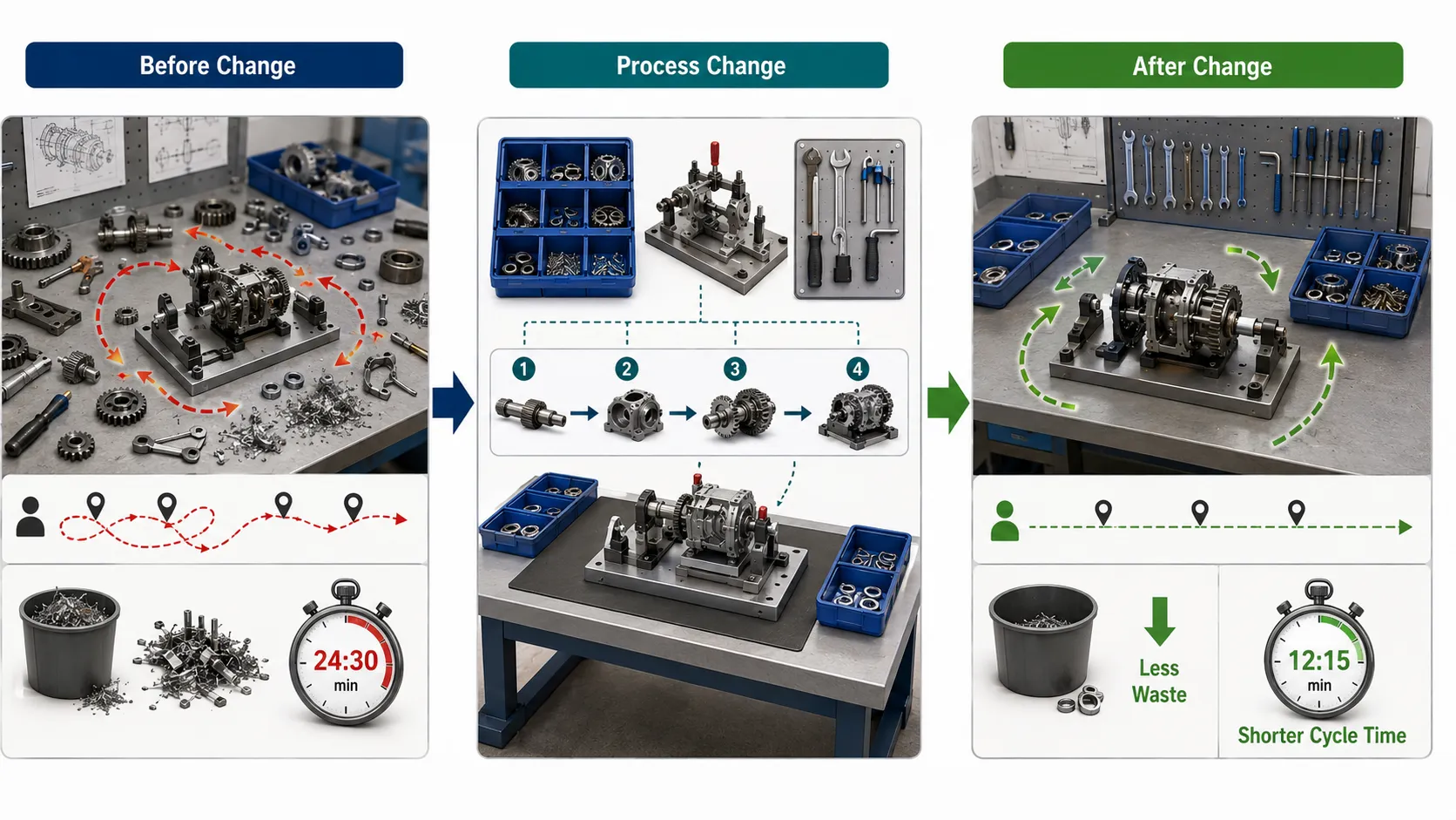
Understanding Targeted Process Change
A targeted process change is a controlled modification to a specific activity, sequence, resource, parameter, layout or working method within an established production process.
In mechanical assembly, a targeted change may involve:
- Rearranging assembly activities.
- Reducing unnecessary component movement.
- Changing material preparation methods.
- Improving component positioning.
- Introducing standardised assembly sequences.
- Reducing excessive handling.
- Optimising fastener preparation.
- Improving tool accessibility.
- Introducing appropriate fixtures or jigs.
- Combining compatible assembly activities.
- Reducing unnecessary waiting time.
- Improving material presentation.
- Eliminating duplicated inspection activities.
- Reducing avoidable rework.
- Improving workstation layout.
The change should be specific enough to measure its effect and controlled enough to prevent unintended consequences.
Key Definitions and Concepts
| Term | Definition | Mechanical Assembly Application |
|---|---|---|
| Process Change | A controlled modification to an existing production activity | Changing the sequence of component installation |
| Assembly Workflow | Ordered sequence of activities used to construct or complete a mechanical product | Component preparation, positioning, fastening and inspection |
| Material Waste | Material consumed without contributing useful value to the finished product | Excessive cutting, damaged parts or unnecessary consumables |
| Cycle Time | Time required to complete a defined production activity or unit | Time from assembly start to completed inspection |
| Value-Added Activity | Activity that directly contributes to the required product function or transformation | Correctly installing and securing a component |
| Non-Value-Added Activity | Activity that consumes resources without directly improving the product | Unnecessary movement or waiting |
| Process Mapping | Visual or structured representation of process activities | Mapping every assembly step from preparation to release |
| Baseline | Measured starting condition before an improvement | Current average assembly time |
| Takt Time | Required production pace to meet demand | Target time per completed assembly |
| Rework | Additional work needed to correct a non-conforming assembly | Reinstalling an incorrectly positioned component |
| Scrap | Material or component rejected as unsuitable for use | Damaged component discarded after assembly |
| Material Yield | Proportion of supplied material converted into acceptable product | Percentage of purchased material incorporated into assemblies |
| First-Pass Yield | Percentage of units meeting requirements without rework | Assemblies accepted at initial inspection |
| Bottleneck | Process stage limiting overall production flow | Slow fastening or inspection operation |
| Standard Work | Defined and controlled method for performing an activity | Approved sequence for assembling a mechanical module |
| Process Capability | Ability of a stable process to consistently meet requirements | Ability to achieve required assembly dimensions |
| Change Validation | Evidence that a process change achieves its intended result | Demonstrating reduced cycle time without increased defects |
| Continuous Improvement | Structured ongoing effort to improve process performance | Repeated reduction of waste and variation |
| Root Cause | Fundamental reason a waste or inefficiency occurs | Poor component layout causing repeated handling |
Why Material Waste and Cycle Time Should Be Analysed Together
Material waste and cycle time are often connected.
For example, an inefficient cutting and preparation process may:
- Consume excessive material.
- Create additional component handling.
- Increase preparation time.
- Produce more scrap.
- Require additional inspection.
- Increase rework.
- Extend the overall assembly cycle.
Likewise, an inefficient assembly sequence may cause:
- Repeated component movement.
- Excessive temporary fastening.
- Incorrect installation.
- Additional disassembly.
- Material damage.
- Rework.
Therefore, the engineering objective should be to identify process activities that consume both material and time without producing additional functional value.
Establishing the Baseline
No process change should be implemented before establishing a reliable baseline.
The baseline should describe the current process under representative production conditions.
Useful baseline measures include:
- Average cycle time.
- Minimum cycle time.
- Maximum cycle time.
- Material consumption per assembly.
- Material scrap per assembly.
- Rework percentage.
- First-pass yield.
- Assembly defects.
- Labour time.
- Tool usage.
- Waiting time.
- Internal transport time.
- Inspection time.
The baseline provides the reference against which the proposed process change can be evaluated.
Identifying Material Waste
Material waste should be measured rather than estimated.
Potential waste sources include:
Cutting Waste
Material may be lost through:
- Excessive cutting allowances.
- Inefficient cutting patterns.
- Incorrect measurements.
- Poor nesting.
- Damaged material.
Component Damage
Components may become unusable because of:
- Incorrect handling.
- Improper storage.
- Incorrect tooling.
- Excessive force.
- Contamination.
Consumable Waste
Consumables may include:
- Welding consumables.
- Sealants.
- Lubricants.
- Adhesives.
- Fasteners.
- Abrasives.
Excessive or incorrect application can increase waste.
Rework-Related Waste
Incorrect assembly can require:
- Replacement components.
- Additional consumables.
- Additional cleaning.
- Additional machining.
- Additional inspection.
This type of waste is particularly important because it may also increase cycle time.
Identifying Cycle-Time Losses
Cycle time should be broken down into individual activities.
A typical mechanical assembly workflow might contain:
- Material retrieval.
- Component identification.
- Component inspection.
- Preparation.
- Positioning.
- Alignment.
- Fastening.
- Adjustment.
- Functional checking.
- Final inspection.
- Documentation.
- Transfer to the next stage.
Each activity should be measured where practical.
Value-Added and Non-Value-Added Activities
An engineering review should distinguish between activities that directly contribute to the product and activities that consume resources without adding equivalent value.
Examples of potential non-value-added activities include:
- Searching for tools.
- Waiting for components.
- Repeated movement between workstations.
- Duplicate data entry.
- Unnecessary component handling.
- Repeated measurement caused by poor preparation.
- Correcting preventable assembly errors.
However, an activity should not be removed merely because it appears non-value-added.
Some inspection and verification activities are essential for quality and safety.
Process Mapping
A process map helps visualise the entire workflow.
A simplified assembly sequence may be represented as:
Material receipt
↓
Component verification
↓
Preparation
↓
Sub-assembly
↓
Positioning
↓
Fastening
↓
Alignment
↓
Functional check
↓
Final inspection
↓
Release
The engineering team can then examine where:
- Material is lost.
- Time is spent waiting.
- Errors occur.
- Rework begins.
- Bottlenecks develop.
Calculating Material Waste
A simple material-waste calculation can be expressed as:
Material Waste = Material Input − Material Incorporated into Acceptable Product
For example:
Material supplied = 12 kg
Material incorporated into acceptable assembly = 10.8 kg
Material waste = 12 − 10.8
Material waste = 1.2 kg
Waste percentage:
1.2 ÷ 12 × 100 = 10%
This provides a measurable baseline.
Calculating Cycle-Time Improvement
Suppose:
Current cycle time = 50 minutes.
Target cycle time = 42 minutes.
Time reduction:
50 − 42 = 8 minutes.
Percentage reduction:
8 ÷ 50 × 100 = 16%
The engineering team should then verify whether the reduction is achieved consistently rather than only during a short trial.
Identifying the Bottleneck
A bottleneck is the stage that restricts the overall production flow.
Examples include:
- Slow component preparation.
- Difficult alignment.
- Manual fastening.
- Repeated adjustment.
- Limited fixture availability.
- Inspection queues.
- Material shortages.
Reducing cycle time at a non-bottleneck stage may have little effect on total production output.
Root-Cause Analysis
Once waste or delay has been identified, the engineering team should determine why it occurs.
Useful questions include:
- Why is material being discarded?
- Why is the component damaged?
- Why does assembly require repeated adjustment?
- Why does the operator wait?
- Why is the same inspection repeated?
- Why does rework occur?
- Why is the workstation difficult to access?
Possible root causes include:
- Poor workstation layout.
- Incorrect material preparation.
- Inadequate fixtures.
- Poor component identification.
- Inconsistent assembly sequence.
- Tool availability problems.
- Inadequate process instructions.
- Poor tolerance management.
Designing the Targeted Change
A targeted change should address a clearly identified cause.
For example:
Problem:
Operators spend excessive time locating fasteners.
Evidence:
Average retrieval time = 6 minutes per assembly.
Cause:
Fasteners are stored away from the assembly workstation.
Potential targeted change:
Introduce organised point-of-use fastener storage.
Expected result:
Reduced movement and retrieval time.
This is more effective than simply instructing operators to “work faster”.
Optimising Material Preparation
Material preparation can have a significant influence on waste.
Potential improvements include:
- Standardised cutting dimensions.
- Improved cutting layouts.
- Controlled allowances.
- Material nesting.
- Component identification before cutting.
- Reuse of suitable offcuts.
- Better storage practices.
Any reuse must remain compatible with technical requirements and traceability controls.
Optimising Assembly Sequence
Assembly sequence can significantly influence cycle time.
A poor sequence may require:
- Repeated removal and installation.
- Difficult access.
- Repositioning.
- Temporary fastening.
- Repeated alignment.
A revised sequence may reduce these activities.
For example:
Instead of installing a component before an inaccessible fastener is positioned, the sequence can be rearranged so that the fastener is installed while access is unrestricted.
The revised sequence should be validated against the engineering requirements.
Improving Workstation Layout
Poor layout creates unnecessary motion.
A workstation improvement may position:
- Frequently used tools near the operator.
- Components in logical sequence.
- Fasteners at point of use.
- Inspection equipment within convenient reach.
- Documentation where it can be accessed without leaving the workstation.
The objective is not simply convenience. Reduced unnecessary movement can reduce cycle time and fatigue while improving process consistency.
Fixtures and Jigs
Appropriate fixtures can improve:
- Positioning.
- Alignment.
- Repeatability.
- Assembly speed.
- Operator consistency.
A fixture may eliminate repeated manual alignment activities.
However, fixtures should be assessed to ensure they do not:
- Damage components.
- Introduce unwanted stresses.
- Restrict required inspection.
- Create safety risks.
- Prevent correct assembly.
Standardising Assembly Work
Once an improved method is validated, standard work should define:
- Assembly sequence.
- Required tools.
- Component orientation.
- Fastening sequence.
- Inspection points.
- Acceptance criteria.
- Material handling requirements.
Standardisation reduces unnecessary variation between operators and shifts.
Reducing Rework
Rework is one of the most important hidden contributors to cycle time and material waste.
Common causes include:
- Incorrect component orientation.
- Incorrect fastening.
- Poor alignment.
- Incorrect component selection.
- Damaged parts.
- Incomplete inspection.
- Incorrect sequence.
Preventive controls should be introduced where practical.
First-Pass Yield
First-pass yield measures the percentage of assemblies that pass the required process without rework.
For example:
100 assemblies produced.
92 accepted first time.
First-pass yield:
92%.
If a process change increases first-pass yield from 92% to 97% while also reducing cycle time, the improvement is more meaningful than cycle-time reduction alone.
Practical Example: Mechanical Pump Assembly
A pump assembly line currently requires 65 minutes per unit.
Historical analysis shows:
- 8 minutes spent retrieving components.
- 7 minutes spent on repeated alignment.
- 5 minutes spent correcting fastener positioning.
- 45 minutes of essential assembly and inspection.
Material records also show increased fastener waste due to incorrect preparation and handling.
The engineering team identifies three targeted changes:
- Point-of-use component storage.
- Improved alignment fixture.
- Standardised fastener preparation.
The objective is to reduce non-value-added time without removing essential quality controls.
Trial Implementation
The proposed change should initially be tested under controlled conditions.
A suitable trial may include:
- Defined number of assemblies.
- Defined operators.
- Defined materials.
- Same inspection criteria.
- Same product specification.
- Measured cycle time.
- Measured material consumption.
- Recorded defects.
This provides comparable before-and-after evidence.
Example Trial Data
| Measure | Before Change | After Change | Improvement |
|---|---|---|---|
| Average cycle time | 65 min | 55 min | 10 min |
| Material waste | 8.5% | 5.5% | 3 percentage points |
| First-pass yield | 92% | 96% | 4 percentage points |
| Rework rate | 8% | 4% | 4 percentage points |
| Component damage | 5 cases | 2 cases | Reduced |
| Assembly output | 7.4/day | 8.7/day | Increased |
These figures are illustrative and would need to be replaced with actual production data in a workplace improvement project.
Controlling the Process Change
The process change should be controlled through an appropriate change-management process.
This may include:
- Defined change proposal.
- Technical review.
- Risk assessment.
- Trial approval.
- Inspection requirements.
- Operator briefing.
- Controlled implementation.
- Performance monitoring.
- Final approval.
Quality Controls During Implementation
Quality controls should remain active during the trial.
Monitor:
- Dimensional conformity.
- Fastening quality.
- Alignment.
- Component condition.
- Functional performance.
- Inspection results.
- Defect rates.
A cycle-time reduction should never be accepted if it results in unacceptable quality deterioration.
Material Waste Monitoring
Material usage should be measured before and after the change.
Potential indicators include:
- Material consumed per unit.
- Scrap per unit.
- Consumable use.
- Damaged component rate.
- Rework material.
- Offcut utilisation.
The objective is to identify whether the process change produces genuine material efficiency.
Cycle-Time Monitoring
Cycle-time data should be collected consistently.
The team should distinguish:
- Processing time.
- Waiting time.
- Movement time.
- Inspection time.
- Rework time.
- Unplanned downtime.
This helps identify whether the improvement is sustainable.
Safety Considerations
A process change should not increase risk simply to reduce cycle time.
Consider:
- Manual handling.
- Tool access.
- Pinch points.
- Ergonomics.
- Stored energy.
- Lifting requirements.
- Hot surfaces.
- Rotating equipment.
- Welding hazards.
- Chemical exposure.
Any new fixture, tool or workflow must be evaluated before implementation.
Maintaining Traceability
Material and component traceability must be preserved.
The process change should not result in:
- Unidentified components.
- Uncontrolled material substitution.
- Lost inspection records.
- Missing batch information.
- Unclear component status.
Efficiency must operate within the organisation’s quality-management framework.
Change Validation
A process change should be validated against predefined acceptance criteria.
Typical criteria may include:
- Cycle time reduced by the targeted amount.
- Material waste reduced.
- First-pass yield maintained or improved.
- No increase in critical defects.
- No adverse effect on component performance.
- Safety requirements maintained.
Statistical Evaluation
Where sufficient data exists, statistical comparison can strengthen the decision.
Potential analyses include:
- Mean cycle time.
- Standard deviation.
- Defect rate.
- Material consumption.
- Process capability.
- Before-and-after comparison.
- Trend analysis.
The objective is to determine whether observed improvement is consistent and meaningful.
Avoiding False Improvements
A short trial can sometimes produce misleading results.
For example:
- Experienced operators may perform the trial.
- Production conditions may be unusually favourable.
- Component complexity may differ.
- Material batches may differ.
- Equipment condition may change.
Therefore, longer-term verification may be required.
Practical Example: Reducing Fastener Waste
A mechanical assembly line uses several hundred fasteners each week.
Historical records show that a significant proportion are discarded because they become contaminated or damaged during preparation.
The team identifies:
- Poor storage location.
- Excessive handling.
- Uncontrolled unpacking.
- Mixed component identification.
A targeted change introduces:
- Point-of-use storage.
- Controlled quantities.
- Clear identification.
- Reduced handling.
The result is lower fastener waste and faster preparation.
Practical Example: Reducing Assembly Movement
An operator repeatedly walks to a shared tool station during assembly.
A time study shows that tool retrieval contributes several minutes to each cycle.
The process change introduces a controlled workstation tool arrangement.
The change reduces movement while ensuring tools remain suitable, inspected and safely stored.
The improvement is measured through:
- Cycle-time reduction.
- Operator movement.
- Defect rate.
- Tool availability.
Practical Example: Alignment Fixture
An assembly requires repeated manual alignment.
Historical data shows that alignment consumes significant time and contributes to rework.
A suitable fixture is designed and tested.
The fixture:
- Holds components in the required position.
- Improves repeatability.
- Reduces manual adjustment.
- Maintains access for required inspection.
The change is validated before full implementation.
Key Benefits of Targeted Process Changes
Reduced Material Waste
Better preparation and handling can reduce unnecessary material consumption.
Shorter Cycle Times
Removing unnecessary movement and waiting can improve throughput.
Improved First-Pass Yield
Better process control can reduce assembly errors.
Lower Rework
Standardised processes reduce avoidable correction.
Improved Productivity
More assemblies can be completed using the same production resources.
Better Material Utilisation
Improved planning can increase the proportion of material converted into acceptable product.
Improved Consistency
Standard work reduces variation between operators.
Reduced Production Cost
Lower scrap, rework and labour time can reduce unit cost.
Improved Process Visibility
Measured workflow performance provides evidence for further improvement.
Risks of Poorly Controlled Process Changes
A poorly designed improvement can cause:
- Increased defects.
- Reduced inspection quality.
- Component damage.
- Increased operator risk.
- Material traceability problems.
- Hidden rework.
- Increased maintenance.
- Reduced reliability.
For this reason, targeted process improvement must always remain evidence-based.
Recommended Process-Change Procedure
Stage 1: Identify the Problem
Define the waste or cycle-time issue.
Stage 2: Collect Baseline Data
Measure material consumption, cycle time and quality.
Stage 3: Map the Workflow
Document each assembly activity.
Stage 4: Identify Root Causes
Determine why waste or delay occurs.
Stage 5: Develop the Change
Design a specific intervention.
Stage 6: Assess Risk
Evaluate quality, safety and operational consequences.
Stage 7: Conduct a Controlled Trial
Implement the change on a defined basis.
Stage 8: Measure Performance
Compare results against baseline.
Stage 9: Validate
Confirm quality and productivity requirements.
Stage 10: Standardise
Update controlled work instructions where appropriate.
Stage 11: Monitor
Continue collecting performance data.
Continuous Improvement Feedback Loop
An effective process-change system can operate as:
Measure
↓
Analyse
↓
Identify waste
↓
Determine root cause
↓
Design targeted change
↓
Trial
↓
Measure results
↓
Validate
↓
Standardise
↓
Monitor
↓
Improve again
This creates a continuous improvement cycle rather than a one-time efficiency project.
Case Study: Mechanical Assembly Workflow Optimisation
Background
A manufacturing facility assembles industrial mechanical modules. Production records show that output is below the planned level even though equipment capacity is adequate.
The QA/QC team reviews:
- Assembly cycle times.
- Material consumption.
- Rework records.
- Component damage.
- Operator movement.
- Inspection results.
Findings
The review identifies three major issues:
- Components are stored too far from the workstation.
- Alignment requires repeated adjustment.
- Fasteners are prepared individually during assembly.
These activities increase time without improving the final mechanical function.
Targeted Change
The engineering team proposes:
- Point-of-use component storage.
- A validated alignment fixture.
- Pre-prepared fastener kits.
Risk Review
The proposed changes are checked for:
- Component identification.
- Fastener traceability.
- Fixture integrity.
- Assembly accuracy.
- Operator safety.
- Inspection access.
Controlled Trial
A defined number of assemblies are completed using the revised workflow.
Measurements include:
- Cycle time.
- Material waste.
- First-pass yield.
- Rework.
- Component damage.
Results
The trial demonstrates:
- Lower average cycle time.
- Reduced unnecessary movement.
- Lower fastener waste.
- Improved first-pass yield.
- No adverse effect on final inspection.
Implementation
The revised workflow is documented and introduced through controlled process management.
Subsequent production data is reviewed to confirm that the improvement is sustained.
Case Study: Material Waste Reduction in Fabricated Assemblies
A fabrication operation produces structural mechanical frames.
Historical material records show significant offcut waste.
The engineering team analyses:
- Standard component lengths.
- Cutting patterns.
- Required tolerances.
- Material batch sizes.
- Offcut dimensions.
A revised material planning method is developed to improve cutting utilisation while maintaining technical requirements.
The trial demonstrates reduced material waste without increasing dimensional defects.
The improvement is then incorporated into controlled planning procedures.
Management of Long-Term Performance
After implementation, the engineering team should continue monitoring:
- Cycle time.
- Material waste.
- First-pass yield.
- Rework.
- Scrap.
- Component reliability.
- Operator feedback.
- Process deviations.
This prevents a temporary improvement from being mistaken for sustainable process optimisation.
Professional Decision-Making Principles
A competent engineering approach should:
- Establish measurable baselines.
- Use real production evidence.
- Identify the true process constraint.
- Distinguish value-added from unnecessary activity.
- Calculate material waste accurately.
- Measure cycle-time components.
- Investigate root causes.
- Design targeted interventions.
- Protect essential quality controls.
- Assess safety implications.
- Conduct controlled trials.
- Validate results.
- Standardise successful changes.
- Monitor long-term performance.
Conclusion
Executing a targeted process change in a mechanical assembly workflow requires a structured combination of engineering analysis, quality control, production measurement and controlled implementation. Material waste and cycle-time losses should first be quantified using reliable production evidence rather than assumptions. Process mapping, time studies, material-use records, inspection results, rework data and operator observations can reveal where unnecessary consumption and delays occur. Once the main causes have been identified, the engineering team can design a focused intervention that addresses the specific source of inefficiency rather than applying broad changes that may create unintended consequences.
A successful process change should improve several dimensions of performance simultaneously. Reducing cycle time is valuable when it increases productive output without increasing defects, rework, equipment stress or safety risk. Similarly, reducing material waste is valuable when material utilisation improves while component quality, dimensional conformity, traceability and functional performance remain controlled. This is why material efficiency and production efficiency should be evaluated alongside first-pass yield, defect rates, rework, scrap and component reliability.
The most effective approach begins with a baseline, followed by workflow analysis and root-cause identification. A targeted change can then be designed around issues such as unnecessary movement, poor material preparation, inefficient component positioning, repeated alignment, excessive handling, poor workstation layout or avoidable rework. Fixtures, jigs, point-of-use material presentation, standardised assembly sequences and improved preparation methods can all contribute to measurable improvement when appropriately designed and validated.
Controlled trials are essential because an apparent improvement in one metric may produce deterioration elsewhere. A process change should therefore be evaluated using predefined acceptance criteria covering cycle time, material consumption, dimensional quality, functional performance, defect levels, first-pass yield, safety and traceability. Where appropriate, statistical analysis can be used to establish whether the observed improvement is consistent and meaningful.
Once a change has been validated, the improved method should be incorporated into controlled production documentation and monitored over time. Continued measurement ensures that the improvement remains effective under normal production conditions rather than only during the initial trial. This creates a sustainable data-driven improvement cycle in which material waste, cycle time, quality and reliability are continually evaluated and improved.
Ultimately, targeted process change is not simply about producing more components in less time. It is about creating a controlled mechanical assembly process that uses materials, equipment, labour and time efficiently while maintaining the required engineering, quality and safety outcomes. When supported by reliable data, structured analysis and disciplined validation, targeted process improvement can reduce waste, shorten cycle times, improve consistency, strengthen component reliability and contribute to long-term manufacturing performance.