
Lesson 1:Apply statistical methods to monitor and control mechanical engineering and manufacturing processes.
Statistical methods provide mechanical engineering and manufacturing teams with a structured way to measure process performance, understand variation, detect abnormal conditions, and maintain consistent quality. In mechanical fabrication, machining, assembly, inspection, and testing environments, relying only on visual checks or individual measurements may not provide sufficient evidence of whether a process remains stable. Statistical analysis allows engineering data to be evaluated systematically, helping identify patterns, trends, process shifts, and unusual variations before they develop into significant quality or reliability problems. Techniques such as statistical process control (SPC), control charts, process capability analysis, sampling, variation analysis, and trend monitoring can therefore support more reliable and evidence-based QA/QC decisions.
Effective statistical process control connects engineering measurements with practical process management. Data from dimensions, tolerances, surface characteristics, material properties, production rates, mechanical test results, defect frequencies, equipment performance, and inspection activities can be analysed to determine whether a manufacturing process is operating consistently within defined requirements. Engineers can distinguish common-cause variation inherent within a stable process from special-cause variation associated with equipment problems, material changes, operator practices, environmental conditions, measurement issues, or process disturbances. This distinction is essential for deciding whether a process should continue under controlled monitoring, undergo investigation, or receive corrective intervention.
A well-designed SPC approach also contributes to manufacturing efficiency, mechanical quality, process capability, and continual improvement. By establishing meaningful baselines and monitoring performance over time, engineering teams can identify emerging problems earlier, reduce unnecessary rework and scrap, improve production consistency, and strengthen confidence in inspection and testing results. Statistical evidence can further support decisions concerning process adjustments, preventive maintenance, quality improvement, and resource allocation. When applied correctly, statistical methods become an important part of modern mechanical engineering quality management, helping organisations achieve greater process stability, repeatability, productivity, and long-term manufacturing performance.
1: Evaluate the Mathematical Principles Behind Statistical Process Control (SPC) to Select the Right Statistical Models for Monitoring Mechanical Production Lines
Statistical Process Control (SPC) provides a mathematical and analytical framework for determining whether a mechanical production process remains stable, predictable, and capable of producing consistent results. In mechanical engineering and manufacturing, production processes naturally contain variation. Machining dimensions may fluctuate slightly, welding characteristics may change between production batches, surface measurements may vary, and mechanical testing results may not produce identical values every time. The purpose of SPC is not to eliminate all variation, because some variation is inherent to the process, but to identify when variation becomes unusual, excessive, or indicative of an underlying process problem.
Selecting an appropriate statistical model therefore requires more than placing measurements on a control chart. Engineers must understand the type of data being collected, the distribution of that data, the sampling method, the measurement system, the process characteristics, the intended engineering requirement, and the consequences of process variation. A suitable SPC model should provide meaningful information about process behaviour without generating excessive false alarms or concealing important process changes. This requires an understanding of mathematical concepts including mean, median, variance, standard deviation, range, probability distributions, sampling, confidence intervals, control limits, specification limits, process capability, and statistical significance.
For mechanical production lines, the correct statistical approach can significantly improve QA/QC performance. It allows engineers to distinguish common-cause variation from special-cause variation, identify trends before components fall outside specification, evaluate process capability, investigate abnormal patterns, and establish evidence-based corrective actions. When statistical models are selected and applied correctly, SPC becomes a proactive engineering tool that supports dimensional accuracy, manufacturing consistency, equipment reliability, defect reduction, process optimisation, and continual improvement.
Understanding Statistical Process Control in Mechanical Engineering
Statistical Process Control is a structured method of using statistical data to monitor process behaviour and identify changes that require investigation or intervention.
In a mechanical manufacturing environment, SPC may be applied to:
Machined component dimensions.
Shaft diameters.
Bore dimensions.
Component thickness.
Surface roughness.
Weld characteristics.
Hardness measurements.
Tensile test results.
Pressure-test results.
Torque measurements.
Assembly dimensions.
Component weights.
Production cycle times.
Defect rates.
Equipment operating parameters.
The underlying principle is that a stable process produces data with a reasonably predictable pattern. When the statistical behaviour changes significantly, engineers can investigate the reason before the problem becomes widespread.
Why Mathematical Principles Matter in SPC
Mathematics provides the basis for determining whether an observed change is meaningful or simply part of normal process variation.
Without mathematical analysis, an engineer might incorrectly conclude that:
Every measurement fluctuation represents a defect.
Every value near a specification limit indicates process failure.
A single unusual result proves equipment malfunction.
A stable process is automatically capable of meeting specifications.
SPC helps prevent these errors by providing quantitative methods for analysing variation.
Key Definitions and Concepts
| Term | Definition | Mechanical Engineering Application |
|---|---|---|
| Statistical Process Control | Statistical method used to monitor and control process behaviour | Monitoring manufacturing stability |
| Population | Complete set of relevant observations | All components produced by a process |
| Sample | Selected observations from a population | Measurements from selected components |
| Mean | Arithmetic average of observations | Average shaft diameter |
| Median | Middle value of ordered observations | Useful for skewed data |
| Range | Difference between maximum and minimum values | Short-term process variation |
| Variance | Measure of squared deviation from the mean | Quantifying process dispersion |
| Standard Deviation | Measure of typical data dispersion around the mean | Evaluating manufacturing consistency |
| Control Limit | Statistically calculated process boundary | Identifying unusual process behaviour |
| Specification Limit | Engineering requirement defining acceptable product limits | Drawing tolerance |
| Common-Cause Variation | Variation inherent in a stable process | Normal machining variation |
| Special-Cause Variation | Variation caused by an identifiable abnormal factor | Tool failure or incorrect setting |
| Process Capability | Ability of a stable process to meet specifications | Evaluating dimensional conformity |
| Process Mean | Central tendency of the process | Average production dimension |
| Sampling | Selecting observations for statistical analysis | Measuring selected components |
| Distribution | Pattern describing how observations are statistically arranged | Normal distribution of dimensions |
| Control Chart | Graphical statistical monitoring tool | Tracking shaft diameter |
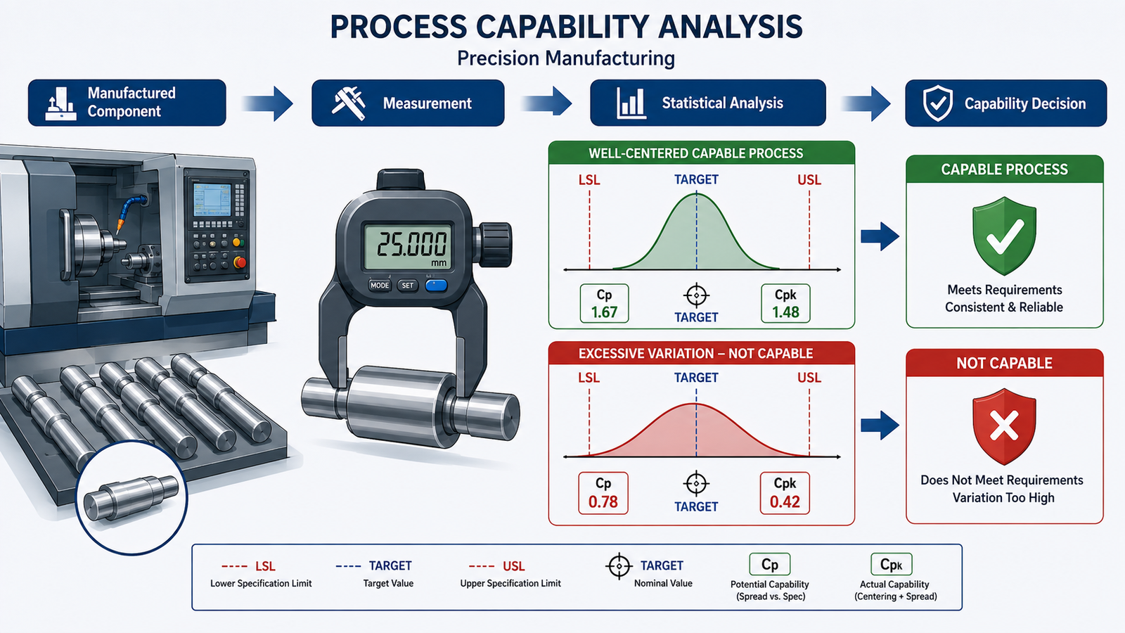
| Cp | Capability index reflecting potential process spread | Comparing variation with tolerance |
| Cpk | Capability index considering process centring | Evaluating actual capability |
| Outlier | Observation unusually distant from other values | Possible measurement or process anomaly |
| Trend | Directional movement in data | Gradual tool wear |
| Statistical Significance | Evidence that an observed difference is unlikely to be random variation | Evaluating process changes |
Understanding Process Variation

Variation is an unavoidable feature of manufacturing.
For example, suppose a machining process is intended to produce shafts with a nominal diameter of 50.00 mm.
Measurements might be:
49.99 mm.
50.01 mm.
50.00 mm.
50.02 mm.
49.98 mm.
Small differences may occur because of:
Tool condition.
Machine vibration.
Material characteristics.
Temperature.
Measurement uncertainty.
Operator interaction.
Cutting conditions.
The engineering objective is to determine whether these differences represent normal process behaviour or indicate a developing problem.
Common-Cause and Special-Cause Variation
Common-Cause Variation
Common-cause variation is produced by factors that are normally present within the process.
Examples include:
Normal machine variation.
Stable material variation.
Routine environmental changes.
Normal measurement variation.
Established process conditions.
If a process contains only common-cause variation, it may be statistically stable.
Special-Cause Variation
Special-cause variation originates from an identifiable abnormal factor.
Examples include:
Broken cutting tools.
Incorrect machine settings.
Sudden material changes.
Sensor malfunction.
Equipment misalignment.
Operator error.
Unexpected temperature changes.
Identifying special causes is one of the major purposes of SPC.
The Arithmetic Mean
The arithmetic mean is one of the most fundamental statistical measures.
It can be calculated using:
Mean = Sum of Observations ÷ Number of Observations
For measurements:
49.98, 50.00, 50.01, 50.02 and 49.99 mm
the mean provides an estimate of the central process location.
The mean is particularly useful when measurements are reasonably symmetric and extreme values are limited.
Practical Importance of the Mean
The process mean helps engineers determine whether a process is centred around its intended target.
For example, a machining process may have a tolerance of:
49.90–50.10 mm
If the average production value gradually shifts towards 50.09 mm, the process may still be within specification but may be becoming poorly centred.
This can indicate the need for process investigation before actual non-conformance occurs.
The Median
The median represents the middle observation after values have been arranged in order.
It can be useful where data contains:
Outliers.
Skewed distributions.
Unusual extreme values.
The median can provide a more robust measure of central tendency in certain datasets.
Range
Range is calculated as:
Range = Maximum Value − Minimum Value
For example:
Maximum = 50.04 mm
Minimum = 49.98 mm
Range:
50.04 − 49.98 = 0.06 mm
Range is useful for examining short-term variation, particularly in subgroup-based control charts.
Variance
Variance measures the average squared deviation from the mean.
Conceptually:
Variance = Average Squared Deviation from Mean
A larger variance indicates greater data dispersion.
In manufacturing, increased variance may indicate:
Tool deterioration.
Machine instability.
Material inconsistency.
Measurement problems.
Changing operating conditions.
Standard Deviation
Standard deviation is the square root of variance.
It is widely used in SPC because it provides a measure of process dispersion in the same units as the original measurement.
For example, if shaft diameter is measured in millimetres, standard deviation is also expressed in millimetres.
A small standard deviation indicates measurements are closely grouped around the mean.
A larger standard deviation indicates greater process variation.
Population and Sample Standard Deviation
Engineers must distinguish between:
Population standard deviation.
Sample standard deviation.
When analysing a sample of production data to estimate population behaviour, the sample standard deviation is commonly used.
For a sample:
s = √[Σ(xᵢ − x̄)² ÷ (n − 1)]
where:
s = sample standard deviation.
xᵢ = individual observation.
x̄ = sample mean.
n = number of observations.
The use of n − 1 rather than n provides an appropriate estimate of population variability from sample data.
Probability Distributions
Statistical models rely on assumptions about how data behaves.
Common distributions encountered in engineering analysis include:
Normal distribution.
Binomial distribution.
Poisson distribution.
Exponential distribution.
The correct model depends on the nature of the data.
Normal Distribution
The normal distribution is particularly important in mechanical manufacturing because many dimensional measurements may approximate a bell-shaped distribution when a stable process is operating under consistent conditions.
A normal distribution is characterised by:
Central mean.
Symmetrical shape.
Predictable dispersion.
Approximately:
68% of observations fall within ±1 standard deviation.
95% fall within ±2 standard deviations.
99.7% fall within ±3 standard deviations.
These values are useful for understanding process dispersion, although engineers should not assume every manufacturing dataset is normally distributed.
Importance of Distribution Testing
Before applying a statistical model, engineers should examine whether its assumptions are reasonable.
Potential methods include:
Histograms.
Probability plots.
Statistical tests.
Box plots.
Distribution analysis.
A model that assumes normality may produce misleading conclusions if the underlying data is strongly skewed.
Sampling Principles
SPC commonly uses samples rather than measuring every component.
Sampling should consider:
Sample size.
Sampling frequency.
Production sequence.
Machine condition.
Shift changes.
Material batches.
Tool changes.
Poor sampling can conceal important process changes.
Rational Subgrouping
Rational subgrouping means grouping observations in a way that helps identify within-process and between-process variation.
For example, five consecutive components may form one subgroup.
This can help determine whether variation occurs:
Within a short production period.
Between different production periods.
After tool changes.
Between shifts.
Correct subgroup selection is important for meaningful control-chart interpretation.
Control Charts
Control charts are graphical tools used to monitor process behaviour over time.
They normally contain:
Centre line.
Upper control limit.
Lower control limit.
Individual process observations or subgroup statistics.
The centre line often represents the process average.
The control limits represent statistically derived boundaries based on expected process variation.
Control Limits Versus Specification Limits
This distinction is fundamental.
Control limits describe statistical process behaviour.
Specification limits describe engineering requirements.
For example:
Lower Specification Limit = 49.90 mm.
Upper Specification Limit = 50.10 mm.
These values may come from a drawing or technical requirement.
Control limits, however, are calculated from process data.
A process can therefore be statistically stable while producing components outside specification.
Conversely, a process can produce measurements within specification while showing statistical instability.
X-Bar Control Charts
An X-bar chart is commonly used to monitor the average of subgroups.
It is useful when:
Measurements are continuous.
Samples are collected in subgroups.
Process centring is important.
For example, five shaft diameters may be measured every hour and their subgroup average plotted.
R Charts
An R chart monitors subgroup range.
It helps identify changes in short-term within-subgroup variation.
An X-bar chart and R chart may therefore be used together.
The X-bar chart examines process location.
The R chart examines process dispersion.
Individuals and Moving Range Charts
Where sampling frequency is low or subgroup sizes are effectively one, an Individuals and Moving Range chart may be appropriate.
This approach can be useful for:
Expensive components.
Destructive testing.
Low-volume production.
Long production cycles.
Attribute Control Charts
Not all quality information is measured continuously.
Some data is categorical.
Examples include:
Defective versus acceptable.
Pass versus fail.
Number of defects.
Number of non-conforming components.
Potential charts include:
p chart.
np chart.
c chart.
u chart.
The choice depends on the type and structure of the attribute data.
Selecting the Correct SPC Model
A structured selection process should begin by asking:
What type of data is available?
Is the data continuous or attribute-based?
Is sampling individual or subgroup-based?
What is the engineering objective?
Is the process expected to follow a particular distribution?
Is process stability being assessed?
Is process capability being evaluated?
What consequences arise from missed variation?
Statistical Model Selection Matrix
| Data / Objective | Potential Tool | Primary Purpose |
|---|---|---|
| Continuous subgroup measurements | X-bar and R | Monitor mean and short-term variation |
| Continuous subgroup measurements with larger samples | X-bar and S | Monitor mean and standard deviation |
| Individual measurements | Individuals and Moving Range | Monitor low-volume or individual observations |
| Fraction defective | p chart | Monitor proportion defective |
| Number defective | np chart | Monitor count of defective units |
| Defect counts with constant opportunity | c chart | Monitor defect counts |
| Defect rates with varying opportunity | u chart | Monitor defects per unit |
| Process capability | Cp / Cpk | Evaluate capability against specifications |
| Failure-time data | Reliability models | Analyse time-to-failure behaviour |
| Process trends | Trend analysis | Identify directional changes |
Process Capability
Process capability determines whether a stable process can consistently meet specification requirements.
Two important indices are:
Cp.
Cpk.
Cp
A simplified capability index is:
Cp = (USL − LSL) ÷ 6σ
where:
USL = Upper Specification Limit.
LSL = Lower Specification Limit.
σ = Process standard deviation.
Cp assesses potential capability based on process spread.
It does not account for whether the process is centred.
Cpk
Cpk incorporates process centring.
It can be expressed as:
Cpk = minimum of:
(USL − Mean) ÷ 3σ
and
(Mean − LSL) ÷ 3σ
This provides a more realistic indication of actual process capability.
Practical Example of Cp and Cpk
Suppose a machined component has:
USL = 50.10 mm.
LSL = 49.90 mm.
Mean = 50.00 mm.
Standard deviation = 0.02 mm.
Then:
Cp = (50.10 − 49.90) ÷ (6 × 0.02)
Cp = 0.20 ÷ 0.12
Cp ≈ 1.67
Because the process is centred at 50.00 mm, Cpk would also be approximately 1.67.
This indicates relatively strong potential capability under the assumptions of the calculation.
When Cp and Cpk Differ
Consider a process with the same variation but a mean of 50.07 mm.
The process may still have a relatively strong Cp, because its spread has not changed.
However, Cpk will decrease because the process is closer to the upper specification limit.
This distinction is important.
A process may have low variation but poor centring.
Control Charts and Process Capability
These tools answer different questions.
Control charts ask:
“Is the process statistically stable?”
Capability analysis asks:
“Can the stable process meet the specification?”
Capability analysis should generally be interpreted after process stability has been established.
Control Chart Patterns
Engineers should look for more than individual points outside control limits.
Potential warning patterns include:
Sustained upward trends.
Sustained downward trends.
Long runs on one side of the centre line.
Sudden shifts.
Cyclic behaviour.
Increasing spread.
Decreasing spread.
These patterns may indicate process changes.
Trend Detection
Suppose shaft diameter measurements increase gradually over several hours.
Possible causes include:
Tool wear.
Thermal growth.
Machine drift.
Fixture movement.
The process may still be within specification.
SPC provides an opportunity to investigate before non-conformance occurs.
Outliers
An outlier is a value significantly different from the surrounding observations.
An outlier may result from:
Measurement error.
Recording error.
Equipment disturbance.
Material anomaly.
Genuine special cause.
It should not automatically be deleted.
The engineering team should investigate its origin.
Measurement System Considerations
SPC depends on measurement quality.
If a measurement system produces excessive variation, the control chart may incorrectly indicate process instability.
Measurement-system considerations include:
Calibration.
Resolution.
Repeatability.
Reproducibility.
Gauge capability.
Measurement environment.
Measurement System Analysis
Before relying heavily on SPC data, organisations should establish that the measurement system is suitable.
A measurement system should:
Have appropriate accuracy.
Have sufficient resolution.
Be properly calibrated.
Be consistently applied.
Be suitable for the tolerance being measured.
Statistical Significance Versus Engineering Significance
A statistically significant difference is not necessarily an engineeringly significant problem.
For example, a very large dataset may detect a tiny dimensional shift that has no practical effect on component function.
Conversely, a small but critical deviation may have major engineering consequences.
Professional judgement must therefore consider both statistical and engineering significance.
Choosing Sample Size
Larger samples generally provide more information but require:
More measurement time.
More inspection resources.
Greater data handling.
Smaller samples may be more economical but may provide less statistical confidence.
Sample size should reflect:
Process variability.
Product criticality.
Production volume.
Inspection cost.
Failure consequence.
Confidence Intervals
Confidence intervals provide a range of plausible values for a population parameter based on sample data.
For example, engineers may estimate:
Population mean.
Population proportion.
Process performance.
Confidence intervals help communicate uncertainty rather than presenting estimates as exact facts.
Hypothesis Testing
Hypothesis testing can help determine whether an observed process change is likely to represent a meaningful difference.
Potential applications include:
Comparing two production periods.
Comparing machines.
Evaluating a process modification.
Assessing supplier batches.
The method should be selected according to the data and analytical objective.
Practical Example: Comparing Two Machining Processes
A manufacturer introduces a new machining setup.
Engineers want to determine whether the new setup changes shaft diameter variation.
They collect samples from:
Existing process.
New process.
The analysis considers:
Mean.
Standard deviation.
Distribution.
Capability.
Control-chart behaviour.
The objective is not simply to identify which mean is lower, but to determine whether the new process provides a statistically and practically meaningful improvement.
SPC and Manufacturing Defects
SPC can identify changes associated with:
Increased dimensional defects.
Surface-quality problems.
Welding variation.
Incorrect assembly.
Heat-treatment inconsistencies.
Material variability.
However, SPC does not identify root causes automatically.
It identifies statistical evidence that supports investigation.
Root-Cause Investigation
Once abnormal variation is identified, engineers may investigate:
Machine settings.
Tool condition.
Material batch.
Operator practices.
Environmental conditions.
Calibration.
Maintenance history.
Process sequence.
Statistical evidence should guide investigation rather than replace engineering analysis.
Practical Example: Tool Wear
A machining line produces shafts.
The X-bar chart shows a gradual upward trend in average diameter.
The R chart remains stable.
This pattern suggests that process centring may be shifting while short-term variation remains relatively stable.
A likely area for investigation is gradual tool wear or machine drift.
The engineering team can then:
Inspect the cutting tool.
Verify machine settings.
Check temperature.
Review maintenance history.
Adjust the process if justified.
Practical Example: Increasing Process Variation
A component thickness process shows:
Increasing range.
Wider distribution.
More frequent control-chart signals.
Possible causes include:
Tool instability.
Material inconsistency.
Fixture problems.
Measurement issues.
The engineering team should investigate before assuming a single cause.
SPC for Welding Processes
SPC can also support welding-related process monitoring where measurable variables are available.
Potential parameters include:
Weld dimensions.
Heat input.
Current.
Voltage.
Travel speed.
Defect frequency.
Statistical analysis can identify process drift and support consistent welding quality.
SPC in Mechanical Testing
Mechanical testing may generate:
Tensile strength.
Yield strength.
Hardness.
Impact results.
Pressure-test values.
Fatigue performance.
SPC can identify whether testing results remain statistically consistent.
However, test-system variation should be separated from actual material or component variation.
Mathematical Model Selection Procedure
Step 1: Define the Engineering Objective
Determine what needs to be monitored.
Step 2: Identify Data Type
Determine whether data is:
Continuous.
Attribute.
Count-based.
Time-based.
Step 3: Assess Data Distribution
Examine whether the data approximates an appropriate statistical distribution.
Step 4: Determine Sampling Structure
Identify:
Individual observations.
Rational subgroups.
Batch samples.
Step 5: Assess Measurement Quality
Confirm calibration and measurement capability.
Step 6: Select Statistical Method
Choose an appropriate control chart or model.
Step 7: Establish Baseline
Calculate relevant central tendency and variation measures.
Step 8: Calculate Control Limits
Use appropriate statistical formulas.
Step 9: Monitor Process Behaviour
Track observations over time.
Step 10: Investigate Signals
Identify potential special causes.
Step 11: Evaluate Capability
Where appropriate, calculate Cp and Cpk.
Step 12: Review and Improve
Use statistical evidence to support engineering action.
Key Benefits of Mathematical SPC
Early Problem Detection
Statistical trends can reveal process deterioration before specification failure.
Reduced Defects
Stable processes generally produce more consistent output.
Reduced Scrap and Rework
Early intervention can prevent large quantities of defective components.
Improved Process Capability
Capability analysis identifies whether variation is compatible with specifications.
Better Equipment Management
Statistical trends may reveal tool or equipment deterioration.
Improved QA/QC Decisions
Engineering decisions can be based on objective data.
Better Manufacturing Efficiency
Stable processes reduce unnecessary intervention.
Improved Customer Confidence
Consistent quality strengthens confidence in manufactured products.
Common Errors in SPC Model Selection
Using the Wrong Control Chart
The chart should match the data type.
Confusing Control Limits With Specifications
Statistical limits and engineering limits have different meanings.
Ignoring Measurement Variation
Poor measurement systems can distort process conclusions.
Assuming Normality
Not all engineering data follows a normal distribution.
Using Inappropriate Sampling
Poor sampling can hide process changes.
Deleting Outliers Without Investigation
An unusual observation may contain valuable process information.
Using Capability Indices Before Establishing Stability
Capability calculations may be misleading for unstable processes.
Relying Only on Statistical Results
Engineering judgement remains essential.
Case Study: Selecting an SPC Model for a Mechanical Production Line
Background
A manufacturing facility produces precision shafts for industrial machinery.
The specified diameter is:
49.90–50.10 mm.
The production line measures five consecutive shafts every hour.
Initial Data
The engineering team collects several weeks of measurements.
The data is continuous and naturally grouped into five-unit samples.
The measurement system has been verified as suitable.
Model Selection
Because:
The data is continuous.
Samples contain five observations.
The process mean is important.
Within-subgroup variation is relevant.
The engineering team selects:
X-bar chart for subgroup averages.
R chart for subgroup ranges.
Analysis
The X-bar chart shows a gradual upward movement.
The R chart remains relatively stable.
This indicates that the process average is changing while short-term variation remains comparatively consistent.
Investigation
The team reviews:
Tool condition.
Machine temperature.
Machine settings.
Maintenance records.
Tool wear is identified as a likely contributing factor.
Corrective Action
The maintenance and production teams introduce a controlled tool-replacement strategy.
The process is then monitored again.
Capability Evaluation
After stabilisation, Cp and Cpk are calculated to determine whether the process can consistently meet the dimensional requirements.
Outcome
The process becomes more predictable, reducing the risk of producing shafts near or beyond the specification boundary.
This case illustrates the importance of selecting a statistical model according to data structure rather than simply applying a preferred chart to every process.
Strategic Engineering Use of SPC
At an advanced engineering level, SPC should support broader decision-making.
Statistical evidence can inform:
Process optimisation.
Preventive maintenance.
Equipment replacement.
Tool-life management.
Supplier quality.
Inspection frequency.
Production planning.
Quality improvement.
Linking SPC With QA/QC
SPC can be integrated with:
Inspection plans.
Non-conformance management.
Corrective action.
Calibration systems.
Process audits.
Supplier quality management.
Preventive maintenance.
This creates a connected quality-control system.
Linking SPC With Preventive Maintenance
Statistical trends can indicate equipment deterioration.
For example:
Increasing dimensional variation → potential machine deterioration → engineering investigation → maintenance intervention → restored process stability.
This creates a proactive connection between quality data and equipment maintenance.
Linking SPC With Continuous Improvement
SPC supports the cycle:
Measure → Analyse → Identify → Correct → Verify → Standardise → Monitor
This enables organisations to maintain process improvements rather than relying on one-time corrective actions.
Professional Engineering Judgement
Mathematical models provide evidence, but engineers must interpret that evidence within the actual production environment.
Considerations may include:
Product criticality.
Safety consequences.
Process complexity.
Measurement reliability.
Production conditions.
Equipment condition.
Applicable specifications.
Cost of intervention.
A statistically stable process is not necessarily an acceptable process if its mean is consistently outside the required specification.
Data Governance
Reliable SPC requires controlled data.
Organisations should manage:
Data collection.
Data storage.
Data validation.
Revision control.
Access control.
Calculation methods.
Statistical software.
Reporting.
Incorrect or altered data can compromise the entire analysis.
Use of Statistical Software
Modern engineering teams may use statistical software to:
Generate control charts.
Calculate capability indices.
Analyse distributions.
Identify trends.
Perform hypothesis testing.
Create statistical reports.
However, software output should be reviewed by competent personnel.
The software does not determine whether the selected model is technically appropriate.
Interpreting Software Output
Engineers should verify:
Correct data input.
Correct units.
Correct subgroup structure.
Correct statistical method.
Correct control-chart type.
Correct specification limits.
Appropriate assumptions.
A visually impressive statistical chart can still be technically invalid if the wrong method was selected.
Summary of Model Selection
A practical selection logic can be expressed as:
Data Type → Distribution → Sampling Structure → Engineering Objective → Statistical Model → Control Method → Interpretation → Action
This sequence helps ensure that the statistical approach is appropriate for the actual mechanical production process.
Conclusion
Evaluating the mathematical principles behind Statistical Process Control is essential for selecting appropriate statistical models for mechanical production and manufacturing processes. Mechanical systems naturally contain variation, and effective SPC does not attempt to eliminate every fluctuation. Instead, it establishes a quantitative framework for distinguishing normal process behaviour from unusual changes that may indicate equipment deterioration, tool wear, material variation, measurement problems, incorrect settings, or other special causes.
Understanding mean, range, variance, standard deviation, probability distributions, sampling, control limits, specification limits, process capability, Cp, Cpk, and statistical significance enables engineers to select control methods according to the characteristics of the production data. X-bar and R charts may be appropriate for continuous subgroup measurements, Individuals and Moving Range charts can support individual observations, while p, np, c, and u charts may be appropriate for different forms of attribute and defect data. Capability analysis can then be used to determine whether a stable process is capable of meeting defined engineering specifications.
The strongest SPC systems combine mathematical analysis with practical engineering judgement. Engineers must validate measurement systems, select suitable sampling strategies, understand data distributions, distinguish control limits from specification limits, investigate unusual signals, and consider both statistical and engineering significance. When properly integrated into mechanical QA/QC, SPC provides an evidence-based method for improving manufacturing consistency, reducing defects, detecting process deterioration, controlling variation, supporting preventive maintenance, and strengthening continual improvement. The ultimate objective is not simply to produce statistical charts, but to use reliable engineering data to maintain stable, capable, safe, and efficient mechanical production processes.
2: Calculate Process Capability Indices to Determine if a Mechanical Manufacturing Line Can Consistently Produce Components Within Specified Design Tolerances
Process capability analysis is a fundamental statistical quality-control technique used to determine whether a stable mechanical manufacturing process can consistently produce components within specified engineering tolerances. In mechanical engineering, dimensional accuracy is often critical because small variations in shaft diameter, bore size, wall thickness, flatness, length, concentricity, or other characteristics can affect assembly, load transfer, sealing, alignment, fatigue performance, and overall mechanical reliability. Process capability indices provide a quantitative method for comparing the natural variation and centring of a manufacturing process with the specification limits defined by engineering drawings, approved designs, manufacturing requirements, or applicable technical documentation.
The most widely used capability measures include Cp and Cpk, with additional indices such as Cpm and Pp/Ppk being useful in particular applications. These indices should not be treated simply as numerical scores. Their meaning depends on whether the manufacturing process is statistically stable, whether the measurement system is capable of producing reliable data, whether the sampled data appropriately represents production, and whether the underlying statistical assumptions are reasonable. A process can have a favourable capability index while subsequently becoming unstable, or it can demonstrate statistical stability while being incapable of consistently meeting design tolerances. Professional interpretation therefore requires both mathematical analysis and engineering judgement.
For mechanical QA/QC teams, capability analysis provides valuable evidence for deciding whether a machining, fabrication, forming, casting, assembly, or testing process requires adjustment. It can identify excessive process variation, poor centring, drift towards a specification boundary, or inadequate manufacturing consistency. When integrated with SPC, inspection data, measurement-system analysis, maintenance records, and corrective-action processes, capability analysis supports proactive quality management and helps reduce scrap, rework, non-conforming components, production interruptions, and unnecessary inspection effort.
Understanding Process Capability
Process capability describes the ability of a stable manufacturing process to produce output within specified engineering requirements.
The analysis compares:
Process Variation + Process Centring + Specification Limits
A capable process should have sufficiently low variation and appropriate centring relative to the tolerance range.
For mechanical manufacturing, capability analysis may be applied to:
- Shaft diameters.
- Bore dimensions.
- Component thickness.
- Machined lengths.
- Hole positions.
- Surface measurements.
- Press-fit dimensions.
- Gear dimensions.
- Seal dimensions.
- Heat-treatment characteristics.
- Mechanical test results.
- Assembly clearances.
Key Definitions and Concepts
| Term | Definition | Mechanical Engineering Application |
|---|---|---|
| Process Capability | Ability of a stable process to meet specified requirements | Assessing machining consistency |
| Specification Limit | Engineering boundary defining acceptable product output | Drawing tolerance |
| USL | Upper Specification Limit | Maximum permitted dimension |
| LSL | Lower Specification Limit | Minimum permitted dimension |
| Target | Preferred nominal process value | Design nominal dimension |
| Process Mean | Average measured process output | Average shaft diameter |
| Standard Deviation | Measure of process dispersion | Quantifying dimensional variation |
| Cp | Capability index based on process spread | Evaluating potential capability |
| Cpk | Capability index considering spread and centring | Evaluating actual capability |
| Cpm | Capability measure incorporating target deviation | Assessing variation and target performance |
| Pp | Overall performance index based on observed variation | Long-term performance assessment |
| Ppk | Overall performance index considering centring | Long-term performance and centring |
| Process Stability | Consistent statistical behaviour over time | Requirement before capability interpretation |
| Tolerance | Permitted dimensional or performance variation | Manufacturing requirement |
| Capability Ratio | Relationship between specification width and process spread | Quantifying capability |
| Centring | Position of process mean relative to target or limits | Detecting process offset |
| Variation | Differences between individual process outputs | Manufacturing consistency |
| Sample | Selected measurements representing production | Capability data collection |
| Outlier | Observation unusually different from the dataset | Possible abnormal measurement |
| Baseline | Established reference process condition | Comparing future performance |
Specification Limits in Mechanical Engineering
Specification limits define the acceptable range for a component characteristic.
For example, an engineering drawing may specify:
- Nominal diameter: 50.00 mm.
- Lower specification limit: 49.90 mm.
- Upper specification limit: 50.10 mm.
The total tolerance width is:
USL − LSL
50.10 − 49.90 = 0.20 mm.
This tolerance represents the permitted dimensional range.
Specification Limits Versus Control Limits
This distinction is essential.
Specification limits originate from engineering requirements.
Control limits are calculated from process behaviour.
For example:
- LSL = 49.90 mm.
- USL = 50.10 mm.
These are specification limits.
Control limits might be calculated from process data and could be narrower or wider than the specification range.
A process can therefore be:
- Statistically stable but incapable.
- Statistically stable and capable.
- Statistically unstable but apparently within specification at a particular point in time.
Why Process Stability Comes First
Capability analysis assumes that the process being analysed behaves consistently.
If the process is unstable because of:
- Tool changes.
- Machine faults.
- Material changes.
- Operator adjustments.
- Environmental changes.
- Calibration problems.
then a capability index may combine different process conditions and produce a misleading result.
Therefore, engineers should generally establish statistical stability before relying on capability indices for process decisions.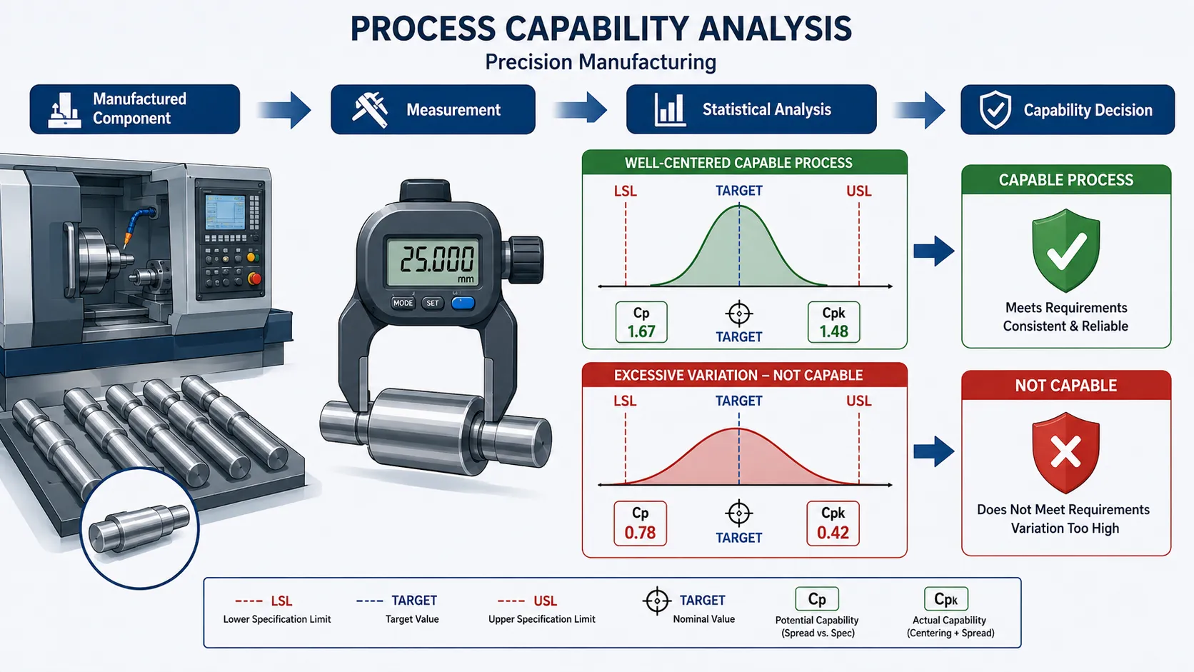
Relationship Between SPC and Capability Analysis
SPC asks:
“Is the process statistically stable and predictable?”
Capability analysis asks:
“Can the stable process meet the engineering specifications?”
This distinction makes SPC and capability analysis complementary rather than interchangeable.
Process Mean
The process mean represents the central tendency of production measurements.
For example, suppose five shaft measurements are:
49.98, 50.01, 50.00, 49.99 and 50.02 mm.
The mean is:
Mean = Sum of Measurements ÷ Number of Measurements
The mean provides an indication of where the process is centred.
Standard Deviation
Standard deviation describes how widely measurements are distributed around the process mean.
A small standard deviation indicates tightly grouped measurements.
A large standard deviation indicates greater process variation.
For capability analysis, standard deviation is particularly important because it determines the estimated process spread.
Cp: Potential Process Capability
Cp compares the width of the specification range with the natural six-standard-deviation spread of the process.
The commonly used formula is:
Cp = (USL − LSL) ÷ 6σ
where:
- USL = Upper Specification Limit.
- LSL = Lower Specification Limit.
- σ = Process standard deviation.
Cp focuses on variation.
It does not account for whether the process mean is centred.
Interpreting Cp
Conceptually:
- Cp below 1.00 indicates that process spread is wider than the specification range.
- Cp around 1.00 indicates that process spread approximately matches the specification width.
- Higher Cp values indicate greater potential capability.
However, organisations may establish their own acceptance criteria depending on product criticality, industry requirements, customer requirements, and risk.
Example of Cp Calculation
Consider a shaft manufacturing process:
- USL = 50.10 mm.
- LSL = 49.90 mm.
- Standard deviation = 0.02 mm.
Then:
Cp = (50.10 − 49.90) ÷ (6 × 0.02)
Cp = 0.20 ÷ 0.12
Cp ≈ 1.67
This indicates that the estimated process spread is considerably narrower than the specification width, assuming the data and statistical assumptions are appropriate.
What Cp Does Not Tell You
Cp does not indicate whether the process is centred.
Consider a process that has very low variation but operates consistently close to the upper specification limit.
It may have a good Cp because the spread is small.
However, if the mean moves too close to the upper limit, actual capability is reduced.
This is why Cpk is important.
Cpk: Actual Process Capability
Cpk accounts for both process variation and process centring.
The commonly used calculation is:
Cpk = Minimum of:
(USL − Mean) ÷ 3σ
and
(Mean − LSL) ÷ 3σ
Cpk therefore identifies the side of the specification range that presents the greater capability limitation.
Why Cpk Is Important
Cpk answers a more practical question:
“How well does the actual process perform relative to the closest specification boundary?”
A process with excellent variation control can still have poor Cpk if its mean is poorly centred.
Example of Cpk Calculation
Consider:
- USL = 50.10 mm.
- LSL = 49.90 mm.
- Mean = 50.07 mm.
- Standard deviation = 0.02 mm.
Upper capability:
(50.10 − 50.07) ÷ (3 × 0.02)
= 0.03 ÷ 0.06
= 0.50
Lower capability:
(50.07 − 49.90) ÷ 0.06
= 0.17 ÷ 0.06
≈ 2.83
Therefore:
Cpk = 0.50
Although the process may have a relatively narrow spread, it is poorly centred towards the upper specification limit.
Comparing Cp and Cpk
The relationship between Cp and Cpk can reveal process centring.
If:
Cp ≈ Cpk
the process may be reasonably centred.
If:
Cp is significantly greater than Cpk
the process may be off-centre.
This provides an important diagnostic indicator.
Process Centring
A well-centred process has its mean located close to the intended target.
For a symmetric tolerance:
LSL = 49.90 mm
Target = 50.00 mm
USL = 50.10 mm
A mean near 50.00 mm indicates good centring.
A mean of 50.08 mm indicates that the process has shifted towards the upper limit.
Target Versus Mean
The engineering target and actual process mean should not be assumed to be identical.
A process can produce:
- Very consistent measurements.
- Low standard deviation.
- High Cp.
Yet still have a mean that is significantly different from the target.
This situation can produce a reduced Cpk.
Cpm and Target Performance
Cpm incorporates both process variation and deviation from the target.
A commonly used form is:
Cpm = (USL − LSL) ÷ [6√(σ² + (Mean − Target)²)]
This index is useful where achieving the target value is particularly important.
It penalises processes that are consistently away from the desired target even if they remain within specification.
Pp and Ppk
Cp and Cpk are commonly associated with within-process variation under capability assumptions.
Pp and Ppk are often used to assess overall observed process performance using overall variation.
Conceptually:
Pp = Specification Width ÷ Overall Process Spread
Ppk = Minimum Upper/Lower Performance Distance ÷ Overall Process Spread
The exact calculation methodology should be controlled within the organisation’s statistical procedure.
Short-Term Capability Versus Long-Term Performance
This distinction is important.
A process may show:
- Strong short-term capability.
- Lower long-term performance.
Long-term data may contain:
- Shift changes.
- Tool replacement.
- Material batches.
- Temperature changes.
- Maintenance interventions.
- Operator changes.
Pp and Ppk can therefore provide useful information about broader observed performance.
Process Capability Data Collection
A capability study should be designed carefully.
The engineering team should define:
- Characteristic being measured.
- Specification limits.
- Target.
- Sampling plan.
- Sample size.
- Production period.
- Equipment condition.
- Measurement method.
- Data exclusion rules.
Sampling Strategy
The sample should represent normal production.
It should ideally cover relevant sources of variation, such as:
- Different shifts.
- Different production periods.
- Normal tool usage.
- Material batches.
- Typical operating conditions.
However, mixing fundamentally different processes without proper analysis can conceal important differences.
Measurement System Capability
Capability analysis depends on measurement accuracy.
If a gauge introduces substantial measurement variation, the observed process variation may be inflated.
This can result in an artificially low capability index.
Before conducting capability analysis, engineers should therefore verify:
- Calibration status.
- Gauge resolution.
- Repeatability.
- Reproducibility.
- Measurement method.
- Environmental conditions.
Measurement Resolution
The measuring instrument must be suitable for the tolerance.
For example, measuring a very narrow engineering tolerance using a low-resolution instrument can produce unreliable capability results.
The measurement system should be sufficiently precise for the engineering decision being made.
Data Screening
Before calculating capability indices, engineers should examine the dataset.
Useful methods include:
- Histogram.
- Box plot.
- Control chart.
- Probability plot.
- Summary statistics.
The purpose is to identify:
- Outliers.
- Non-normality.
- Trends.
- Shifts.
- Clusters.
- Data-entry errors.
Outliers
An outlier should not automatically be removed.
It may represent:
- Measurement error.
- Genuine process failure.
- Special cause.
- Equipment malfunction.
- Material problem.
The reason for the outlier should be investigated and documented.
Normality Considerations
The traditional Cp and Cpk interpretation is commonly associated with approximately normal continuous data.
If the data is significantly non-normal, engineers may need to consider:
- Transformation methods.
- Non-normal capability analysis.
- Alternative statistical models.
The chosen approach should reflect the actual data distribution.
Practical Example: Machined Shaft
A manufacturer produces shafts with:
- Target = 50.00 mm.
- LSL = 49.90 mm.
- USL = 50.10 mm.
Measurements are collected over a controlled production period.
The analysis shows:
- Mean = 50.01 mm.
- Standard deviation = 0.02 mm.
Cp:
0.20 ÷ 0.12 = 1.67
The process mean is close to target.
Therefore, Cpk is also approximately 1.50–1.67 depending on the precise calculation and rounding.
The engineering team concludes that the process has relatively low variation and reasonable centring, subject to the applicable organisational acceptance criterion and stability evidence.
Practical Example: Off-Centre Machining Process
Consider another process:
- Target = 50.00 mm.
- LSL = 49.90 mm.
- USL = 50.10 mm.
- Mean = 50.07 mm.
- Standard deviation = 0.02 mm.
Cp remains approximately:
1.67
But Cpk is approximately:
0.50
This is an important engineering finding.
The process has sufficient potential spread capability but poor centring.
Possible causes may include:
- Incorrect machine offset.
- Tool setting.
- Fixture positioning.
- Machine calibration.
- Thermal effects.
The appropriate response is process-centre correction rather than automatically reducing variation.
Practical Example: Excessive Process Variation
Consider:
- LSL = 49.90 mm.
- USL = 50.10 mm.
- Mean = 50.00 mm.
- Standard deviation = 0.04 mm.
Cp becomes:
0.20 ÷ 0.24
≈ 0.83
The process is centred but its variation is too large relative to the tolerance.
Possible causes include:
- Machine instability.
- Tool wear.
- Material variation.
- Poor fixturing.
- Measurement problems.
The solution should focus on reducing variation.
Practical Example: High Cp but Low Cpk
A manufacturing line reports:
- Cp = 2.00.
- Cpk = 0.70.
This combination suggests that the process has relatively low variation but is significantly off-centre.
A common mistake would be to conclude that the process is highly capable because Cp is high.
The lower Cpk reveals the more important issue.
Practical Example: Low Cp and Low Cpk
Suppose:
- Cp = 0.75.
- Cpk = 0.70.
This indicates that process spread is relatively large compared with the specification range.
The process may also be somewhat off-centre.
The improvement priority should therefore include:
- Reducing variation.
- Reviewing process centring.
- Investigating equipment condition.
- Reviewing measurement quality.
Capability and Engineering Tolerances
Engineering tolerances should come from controlled technical sources, such as:
- Approved engineering drawings.
- Product specifications.
- Manufacturing standards.
- Customer requirements.
- Approved technical documentation.
The capability study should not use arbitrary tolerance limits.
Bilateral and Unilateral Tolerances
Some mechanical characteristics have symmetric tolerances.
Example:
50.00 ± 0.10 mm
This gives:
- LSL = 49.90 mm.
- USL = 50.10 mm.
Other characteristics may have unilateral limits.
For example:
- Minimum thickness = 10.00 mm.
- No specified upper restriction within the defined design range.
Capability analysis must reflect the actual engineering requirement.
Capability for Critical Characteristics
Critical mechanical characteristics may require stronger capability controls.
Examples include:
- Safety-critical dimensions.
- Pressure-boundary characteristics.
- Critical shaft diameters.
- Load-bearing dimensions.
- Precision mating surfaces.
- Components affecting mechanical integrity.
For these characteristics, organisations may establish stricter internal capability targets.
Process Capability and Risk
Capability analysis should be connected to engineering risk.
A modest capability concern on a non-critical decorative dimension may have limited consequences.
The same statistical weakness on a critical pressure-boundary component could have major consequences.
Risk considerations include:
- Safety.
- Mechanical integrity.
- Functional performance.
- Reliability.
- Customer requirements.
- Production consequences.
Capability Study Procedure
Step 1: Identify the Critical Characteristic
Determine which measurement is being assessed.
Step 2: Confirm the Specification
Verify:
- Nominal value.
- LSL.
- USL.
- Target.
Step 3: Validate the Measurement System
Confirm that the measurement process is reliable.
Step 4: Establish Process Stability
Use appropriate control charts or statistical evidence.
Step 5: Collect Representative Data
Capture measurements from normal production.
Step 6: Examine the Data Distribution
Assess shape, outliers and trends.
Step 7: Calculate Process Statistics
Determine:
- Mean.
- Standard deviation.
- Range.
- Other relevant measures.
Step 8: Calculate Cp
Evaluate potential process capability.
Step 9: Calculate Cpk
Evaluate actual capability considering centring.
Step 10: Consider Pp and Ppk
Where appropriate, evaluate broader observed performance.
Step 11: Compare With Acceptance Criteria
Use approved organisational or customer criteria.
Step 12: Determine Engineering Action
Possible actions include:
- Continue monitoring.
- Centre the process.
- Reduce variation.
- Improve equipment condition.
- Review tooling.
- Investigate measurement.
- Implement corrective action.
Interpreting Capability Results
A professional interpretation should answer:
- Is the process stable?
- Is the process centred?
- Is process variation sufficiently small?
- Are specification limits being approached?
- Is the measurement system reliable?
- Does the process meet the applicable capability criterion?
- Is the capability sustained over time?
Capability Improvement Strategies
Reduce Process Variation
Potential actions include:
- Improving machine maintenance.
- Replacing worn tooling.
- Improving fixturing.
- Controlling environmental conditions.
- Improving material consistency.
- Improving process settings.
Improve Process Centring
Potential actions include:
- Correcting machine offsets.
- Adjusting tool settings.
- Reviewing calibration.
- Correcting alignment.
- Reviewing setup procedures.
Capability and Tool Wear
Tool wear can gradually shift the process mean.
For example:
Initial mean = 50.00 mm
Later mean = 50.04 mm
Later mean = 50.07 mm
Even if measurements remain within specification, the trend should be investigated.
Capability analysis can quantify the effect of the shift.
Capability and Machine Maintenance
Mechanical condition can influence process capability.
Potential contributors include:
- Spindle condition.
- Bearing condition.
- Machine alignment.
- Fixture wear.
- Hydraulic instability.
- Temperature variation.
Therefore, a declining Cpk may indicate an engineering maintenance issue rather than solely a production-control issue.
Capability and Supplier Quality
The same methodology can be applied to supplier-produced components.
Organisations may evaluate:
- Dimensional capability.
- Material properties.
- Batch consistency.
- Defect rates.
Supplier capability data can support incoming quality decisions.
Capability and Continuous Improvement
Capability analysis supports the improvement cycle:
Measure → Stabilise → Calculate → Identify → Improve → Verify → Monitor
This allows engineering teams to quantify whether process changes have actually improved performance.
Key Benefits
Improved Dimensional Consistency
Capability analysis identifies whether process variation is appropriate for the tolerance.
Reduced Scrap
Stable and capable processes reduce the production of out-of-tolerance components.
Reduced Rework
Early identification of capability problems supports timely intervention.
Improved Product Reliability
Consistent dimensions contribute to reliable mechanical assemblies.
Better Equipment Management
Capability trends can reveal machine deterioration.
Improved QA/QC Control
Statistical evidence strengthens inspection and quality decisions.
Better Process Optimisation
Engineers can identify whether centring or variation is the dominant issue.
Reduced Cost
Improved process control reduces waste and unplanned corrective work.
Common Errors in Capability Analysis
Calculating Cp Without Cpk
Cp alone may hide poor process centring.
Ignoring Stability
Capability indices can be misleading when the process is unstable.
Using Incorrect Specification Limits
The analysis should use approved engineering requirements.
Ignoring Measurement Variation
Poor measurement systems can distort process capability.
Removing Outliers Without Investigation
Outliers may represent real process problems.
Assuming High Cp Means Good Performance
A high Cp with low Cpk can indicate poor centring.
Mixing Different Processes
Combining data from different machines or conditions may produce meaningless results.
Ignoring Long-Term Variation
A short study may not capture important production changes.
Case Study: Capability Assessment of a Precision Machining Line
Background
A manufacturing facility produces precision sleeves used in a mechanical assembly.
The engineering drawing specifies:
- Target diameter: 75.00 mm.
- LSL: 74.90 mm.
- USL: 75.10 mm.
The production team reports occasional assembly difficulties.
Initial Investigation
QA/QC engineers collect dimensional data from the production line.
The measurement system is reviewed and confirmed suitable.
The process is monitored to establish statistical stability.
Statistical Results
The study produces:
- Mean = 75.06 mm.
- Standard deviation = 0.015 mm.
The specification width is:
75.10 − 74.90 = 0.20 mm.
Cp:
0.20 ÷ (6 × 0.015)
= 0.20 ÷ 0.09
≈ 2.22
This suggests strong potential capability.
Cpk Assessment
Upper capability:
(75.10 − 75.06) ÷ (3 × 0.015)
= 0.04 ÷ 0.045
≈ 0.89
Lower capability:
(75.06 − 74.90) ÷ 0.045
≈ 3.56
Therefore:
Cpk ≈ 0.89
Engineering Interpretation
The process has low variation but is poorly centred towards the upper specification limit.
The high Cp might initially suggest excellent capability, but the lower Cpk identifies a significant centring issue.
Investigation
The team reviews:
- Machine offset.
- Tool condition.
- Fixture setup.
- Thermal conditions.
- Calibration.
- Production settings.
A gradual machine offset shift is identified.
Corrective Action
The engineering team:
- Corrects the machine offset.
- Reviews setup procedures.
- Increases short-term monitoring.
- Repeats the capability study.
Verification
The revised process demonstrates:
- Mean closer to target.
- Stable control-chart behaviour.
- Improved Cpk.
- Reduced risk of upper-limit non-conformance.
Outcome
The organisation improves dimensional consistency without unnecessarily reducing production speed or replacing the entire machine.
Management Interpretation of Capability Results
Senior management should not receive capability indices without context.
A useful report should include:
- Characteristic.
- Specification.
- Sample period.
- Measurement system status.
- Process stability.
- Mean.
- Standard deviation.
- Cp.
- Cpk.
- Acceptance criterion.
- Main finding.
- Recommended action.
Engineering Recommendation Based on Capability
If the process demonstrates low Cp:
Recommend actions focused on reducing variation.
If Cp is high but Cpk is low:
Recommend actions focused on process centring.
If both are strong:
Continue monitoring and maintain process controls.
If capability is uncertain because the process is unstable:
Stabilise the process before making a final capability judgement.
Digital Capability Monitoring
Modern manufacturing systems can calculate capability indicators automatically.
Digital systems may integrate:
- Machine measurements.
- Inspection data.
- SPC charts.
- Capability calculations.
- Alarm systems.
- Production records.
However, automated calculation does not replace engineering review.
Data Traceability
Capability studies should maintain traceability between:
Component → Measurement → Machine → Date → Batch → Operator/Process → Statistical Analysis
This allows abnormal results to be investigated efficiently.
Documentation Requirements
A professional capability study should document:
- Purpose.
- Component.
- Characteristic.
- Specification limits.
- Target.
- Measurement method.
- Sample size.
- Sampling period.
- Statistical method.
- Stability assessment.
- Mean.
- Standard deviation.
- Cp.
- Cpk.
- Interpretation.
- Corrective actions.
- Verification results.
Conclusion
Calculating process capability indices provides mechanical engineering and manufacturing teams with a quantitative method for determining whether a stable production process can consistently produce components within specified design tolerances. Cp measures the relationship between specification width and process variation, while Cpk provides a more complete assessment by considering both process variation and centring. Additional measures such as Cpm, Pp, and Ppk can provide further insight where target performance and longer-term variation are important.
However, capability indices should never be interpreted as isolated numbers. A reliable capability study requires a suitable measurement system, representative sampling, appropriate statistical assumptions, and evidence that the production process is stable. Specification limits must be taken from controlled engineering requirements, while control limits and capability calculations must be derived from actual process behaviour. Engineers must also investigate outliers, trends, shifts, and distribution characteristics before accepting the results.
The practical value of capability analysis lies in identifying the specific nature of a process problem. A low Cp generally points towards excessive variation, whereas a significant difference between Cp and Cpk may indicate poor process centring. These distinctions allow engineering teams to select targeted corrective actions, such as improving tooling, machine alignment, maintenance, process settings, fixturing, calibration, or environmental control. When integrated with SPC, QA/QC inspection, measurement-system analysis, maintenance management, and continual improvement, process capability analysis provides a powerful evidence-based approach for improving mechanical manufacturing consistency, reducing non-conformance, controlling waste, strengthening product reliability, and maintaining production processes within their intended engineering tolerances.
3: Apply Sampling Plans and Probability Techniques to Inspect Large Batches of Incoming Mechanical Parts Without Losing Testing Accuracy
Sampling is an essential quality-control technique for organisations that receive large quantities of mechanical components from internal production facilities, approved suppliers, subcontractors, and external manufacturers. Inspecting every component may be impractical when a delivery contains thousands or tens of thousands of items, particularly when inspection involves dimensional measurement, material verification, mechanical testing, non-destructive testing, or other time-consuming activities. A scientifically designed sampling plan allows a representative portion of a batch to be examined while providing a controlled level of confidence about the quality of the wider population.
For mechanical QA/QC engineers, the objective is not simply to reduce the number of inspections. The objective is to reduce unnecessary inspection effort while maintaining an appropriate level of statistical protection against accepting poor-quality material or rejecting satisfactory batches. Sampling therefore requires careful consideration of population size, sample size, defect risk, acceptable quality levels, confidence, inspection severity, measurement accuracy, lot homogeneity, supplier history, and the consequences of undetected defects. Probability theory provides the mathematical foundation for understanding how likely a sample is to detect defects within the larger population.
A robust incoming inspection programme should therefore combine engineering judgement with statistically defensible sampling methods. The approach should be appropriate to the criticality of the mechanical part, the type of characteristic being inspected, the reliability of the supplier, the inspection method, and the potential consequences of non-conforming material entering production. High-risk pressure-containing, load-bearing, safety-critical, or mechanically essential components may require more stringent inspection or even 100% verification of selected characteristics, whereas lower-risk standard components may be suitable for controlled statistical sampling.
Understanding Sampling in Mechanical QA/QC
A sampling plan defines how units are selected from a larger population and how inspection results are used to make an acceptance decision.
In an incoming mechanical parts environment, the population may consist of:
- 5,000 machined shafts.
- 2,000 bearings.
- 10,000 fasteners.
- 1,500 fabricated brackets.
- 800 precision gears.
- 3,000 mechanical seals.
- 6,000 standard washers.
- 1,000 pressure-related components.
Rather than inspecting every item, an engineer may select a statistically justified sample.
The sample should provide meaningful evidence about the quality of the entire lot.
Key Definitions and Concepts
| Term | Definition | Mechanical QA/QC Application |
|---|---|---|
| Population | Complete group of units under consideration | Entire incoming batch |
| Lot | Defined quantity of similar products considered together | Supplier delivery of shafts |
| Sample | Selected units inspected from the population | Selected components from a delivery |
| Sampling Plan | Defined method for selecting and evaluating samples | Incoming inspection procedure |
| Random Sampling | Selection where each unit has a known opportunity of selection | Random component selection |
| Stratified Sampling | Sampling from defined subgroups | Sampling different production batches |
| Acceptance Sampling | Statistical method used to decide whether a lot is accepted | Supplier batch approval |
| Attribute Sampling | Inspection based on categories such as pass/fail | Defective component count |
| Variable Sampling | Inspection based on numerical measurements | Shaft diameter |
| Defect | Failure to meet a specified requirement | Incorrect dimension |
| Defective Unit | Unit containing one or more defects | Non-conforming bearing |
| AQL | Defined quality level used within an acceptance-sampling scheme | Sampling-plan criterion |
| Acceptance Number | Maximum permitted sample defects for acceptance | Accept/reject decision |
| Rejection Number | Defect count triggering rejection | Lot rejection threshold |
| Confidence | Degree of statistical certainty associated with an estimate | Confidence in batch assessment |
| Risk | Probability and consequence of an undesirable outcome | Risk of accepting poor material |
| Sampling Error | Difference between sample findings and population reality | Sample not representing lot |
| Random Variable | Variable whose outcome is uncertain | Measured shaft diameter |
| Probability | Quantitative expression of likelihood | Probability of detecting defects |
| Lot Homogeneity | Degree to which units share similar characteristics | Same material and production conditions |
| Traceability | Ability to connect sample results to the original lot | Supplier batch identification |
Why Sampling Is Important for Incoming Mechanical Parts
Sampling provides several practical advantages.
It can:
- Reduce inspection time.
- Reduce inspection costs.
- Allow large batches to be assessed efficiently.
- Support consistent acceptance decisions.
- Provide measurable statistical confidence.
- Reduce unnecessary destructive testing.
- Focus inspection resources on higher-risk characteristics.
However, sampling also introduces risk.
A sample may contain only acceptable components even when defective units exist elsewhere in the lot.
This is known as sampling risk.
Sampling Risk
There are two important decision risks.
Producer’s Risk
Producer’s risk is the possibility that an acceptable lot is rejected based on sample results.
This can result in:
- Unnecessary supplier investigation.
- Additional inspection.
- Delayed material release.
- Increased costs.
- Disruption to production.
Consumer’s Risk
Consumer’s risk is the possibility that a poor-quality lot is accepted.
This can result in:
- Defective components entering production.
- Rework.
- Equipment failure.
- Increased maintenance.
- Mechanical integrity concerns.
- Safety risks.
For critical mechanical components, consumer risk may be particularly important.
Probability and Sampling
Probability provides the mathematical basis for understanding the likelihood that a sample will identify defects.
If a population contains a certain proportion of defective units, the probability of finding at least one defective unit generally increases as the sample size increases.
For independent selection with replacement or as a simplified approximation for large populations:
Probability of no defective units ≈ (1 − p)ⁿ
where:
- p = proportion defective.
- n = sample size.
Therefore:
Probability of detecting at least one defective unit ≈ 1 − (1 − p)ⁿ
This formula provides an intuitive demonstration of the relationship between defect prevalence and sample size.
Practical Probability Example
Suppose an incoming batch has an assumed defect proportion of 5%.
Therefore:
p = 0.05
If five components are sampled:
Probability of no defect ≈
(1 − 0.05)⁵
= 0.95⁵
≈ 0.774
Therefore, probability of detecting at least one defect is approximately:
1 − 0.774 = 0.226
or approximately 22.6%.
This demonstrates that a very small sample may have limited power to detect defects.
Increasing Sample Size
If the sample size increases to 20:
Probability of no defect ≈
0.95²⁰
≈ 0.358
Probability of detecting at least one defect:
1 − 0.358 = 0.642
or approximately 64.2%.
The probability of detecting at least one defect has increased substantially.
This illustrates why sample size matters.
Important Limitation of the Simple Probability Model
The simplified formula assumes conditions that may not exist in an actual incoming batch.
Real sampling may involve:
- Sampling without replacement.
- Finite population size.
- Non-random selection.
- Clustered defects.
- Multiple defect categories.
For finite populations, the hypergeometric distribution may be more appropriate.
Hypergeometric Distribution
When sampling without replacement from a finite lot, the hypergeometric distribution can provide a more accurate probability model.
For example, suppose:
- Population = 1,000 components.
- Defective components = 50.
- Sample = 20 components.
The probability of selecting a specific number of defective components can be modelled using the hypergeometric distribution.
Conceptually:
P(X = k) = [C(K,k) × C(N−K,n−k)] ÷ C(N,n)
where:
- N = population size.
- K = number of defective units.
- n = sample size.
- k = defective units selected.
- C = combination function.
This is particularly relevant when the sample is a meaningful fraction of the total population.
Random Sampling
Random sampling is one of the strongest basic methods for reducing selection bias.
Each unit should have an appropriate opportunity for selection.
For example, if a delivery contains 5,000 shafts, the inspector should not simply select the first 20 accessible components.
Instead, selection may be based on:
- Random numbers.
- Randomised inventory positions.
- Systematic selection with a random starting point.
- Controlled digital sampling.
Why Convenience Sampling Is Weak
Convenience sampling may accidentally select:
- The easiest components to access.
- Components from the same pallet.
- Components at the top of a container.
- Components from the same production sequence.
If defects are clustered elsewhere, the sample may fail to represent the full lot.
Stratified Sampling
Stratified sampling divides the population into meaningful subgroups.
For example, an incoming batch may contain components produced across:
- Three manufacturing dates.
- Two production lines.
- Four material batches.
Instead of sampling only one subgroup, engineers may sample across each relevant stratum.
This can improve representation when meaningful differences exist between subgroups.
Systematic Sampling
Systematic sampling selects units at regular intervals.
For example:
Population = 1,000 units
Required sample = 20 units
Sampling interval:
1,000 ÷ 20 = 50
A random starting position is selected, followed by every 50th unit.
Systematic sampling can be practical in organised production or storage environments.
However, engineers should ensure that periodic production patterns do not align with the sampling interval.
Acceptance Sampling
Acceptance sampling is used to determine whether a lot should be accepted or rejected based on a sample.
A basic plan may specify:
- Sample size.
- Inspection method.
- Acceptance number.
- Rejection number.
For example:
Sample size = 50
Acceptance number = 1
Rejection number = 2
If no more than one defective unit is found, the lot may be accepted under the defined plan.
If two or more are found, the lot may be rejected.
The actual acceptance criteria must come from the approved sampling procedure or applicable standard.
Attribute Sampling
Attribute sampling classifies inspection results.
Examples include:
- Acceptable / defective.
- Pass / fail.
- Conforming / non-conforming.
Attribute sampling is useful when the engineering question is categorical.
Examples:
- Is the component correctly marked?
- Is the thread damaged?
- Is the surface visibly defective?
- Does the part meet the acceptance criterion?
Variable Sampling
Variable sampling uses measured numerical values.
Examples include:
- Diameter.
- Length.
- Thickness.
- Hardness.
- Pressure.
- Weight.
- Surface roughness.
Variable sampling can provide more information from each measurement than simple pass/fail classification.
Attribute Versus Variable Sampling
A variable measurement may tell an engineer:
“The average diameter is 50.02 mm with a standard deviation of 0.015 mm.”
An attribute inspection may simply record:
“Conforming.”
The variable approach can provide deeper statistical information but requires suitable measurement equipment and analytical methods.
Acceptance Quality Level
AQL is commonly used within formal acceptance-sampling systems to represent a specified quality level associated with an acceptance plan.
It should not be interpreted as permission to manufacture or supply a fixed percentage of defective components.
AQL is a parameter used within a defined statistical sampling methodology.
Inspection Levels
Sampling systems may use different inspection levels depending on:
- Lot size.
- Required discrimination.
- Inspection cost.
- Product criticality.
The organisation’s approved sampling procedure should define how inspection levels are selected.
Normal, Reduced and Tightened Inspection
Some sampling systems allow inspection severity to change according to supplier performance.
Possible approaches include:
- Normal inspection.
- Reduced inspection.
- Tightened inspection.
For example, repeated supplier failures may trigger tightened inspection.
Strong historical supplier performance may support reduced inspection where permitted by the approved quality system.
Supplier History and Sampling
Historical performance can be useful in determining inspection strategy.
Relevant information may include:
- Previous rejection rates.
- Non-conformance frequency.
- Corrective-action effectiveness.
- Supplier audit findings.
- Delivery consistency.
- Material traceability performance.
However, historical performance should not be used to override critical technical requirements.
Risk-Based Sampling
Sampling should reflect the consequences of failure.
High-risk components may justify:
- Larger samples.
- More stringent acceptance criteria.
- Additional testing.
- 100% inspection of critical characteristics.
- Increased supplier surveillance.
Lower-risk standard components may be suitable for less intensive sampling where justified.
Mechanical Criticality
Examples of potentially high-criticality components include:
- Pressure-containing components.
- Load-bearing components.
- Safety-critical shafts.
- Critical fasteners.
- Rotating equipment components.
- Components essential to mechanical containment.
The criticality assessment should consider both probability and consequence.
Destructive Testing and Sampling
Sampling is particularly valuable where testing is destructive.
For example:
- Tensile testing.
- Hardness testing involving permanent marks.
- Sectioning.
- Metallographic examination.
Testing every component may make the entire batch unusable.
A statistically justified sample can provide quality evidence while preserving the majority of the batch.
Non-Destructive Testing and Sampling
NDT methods may include:
- Ultrasonic testing.
- Radiographic testing.
- Magnetic particle testing.
- Dye penetrant testing.
Although NDT does not normally destroy the component, inspection capacity and cost can still make 100% testing impractical.
Sampling can therefore support efficient inspection where the risk assessment and governing requirements permit it.
Sampling and Measurement Accuracy
A statistically sound sampling plan cannot compensate for poor measurement.
Inspection equipment should be:
- Calibrated.
- Suitable for the characteristic.
- Correctly used.
- Appropriately resolved.
- Maintained.
The measurement process should be capable of distinguishing conforming and non-conforming parts.
Sample Size Considerations
Sample size may be influenced by:
- Lot size.
- Desired confidence.
- Defect level of interest.
- Acceptable risk.
- Product criticality.
- Inspection cost.
- Testing method.
- Supplier history.
There is no universal sample size that is appropriate for every mechanical batch.
Confidence
Confidence describes how strongly the statistical evidence supports an inference about the wider population.
Higher confidence generally requires:
- Larger sample sizes.
- Stronger sampling design.
- Reliable measurements.
However, confidence does not guarantee that every unit in the population is conforming.
Confidence and Defect Detection
Suppose an engineer wants a high probability of detecting defects if the defect rate exceeds a particular threshold.
The required sample size will depend on:
- Target defect rate.
- Desired detection probability.
- Population size.
- Sampling method.
This provides a more defensible basis for sample-size selection than simply choosing an arbitrary number.
Practical Example: Incoming Shaft Batch
A supplier delivers 10,000 precision shafts.
The engineering specification identifies:
- Diameter.
- Length.
- Surface condition.
- Material certification.
The QA/QC team develops an approved sampling plan.
Inspection Process
- Verify lot identity.
- Confirm supplier documentation.
- Confirm material traceability.
- Select representative samples.
- Measure critical dimensions.
- Record results.
- Apply acceptance criteria.
- Document the decision.
The sampling plan prevents the inspector from selecting only visually convenient parts.
Practical Example: Fastener Batch
A delivery contains 20,000 mechanical fasteners.
The organisation classifies the fasteners as a standard component with established supplier performance.
The approved sampling system specifies the sample size and acceptance criteria.
The inspector:
- Verifies batch number.
- Confirms material documentation.
- Checks identification.
- Selects random samples.
- Checks dimensions.
- Inspects threads.
- Reviews surface condition.
- Records defects.
The batch is accepted only when the results satisfy the defined acceptance criteria.
Practical Example: High-Risk Pressure Component
A supplier delivers a batch of pressure-containing mechanical components.
Although sampling could reduce inspection workload, the engineering risk is substantially higher.
The quality team considers:
- Failure consequence.
- Applicable technical requirements.
- Supplier history.
- Material traceability.
- NDT requirements.
- Critical dimensions.
The final inspection strategy may require significantly greater inspection coverage or 100% examination of specified characteristics.
This demonstrates why statistical sampling should never be applied mechanically without considering engineering risk.
Sampling Procedure for Incoming Mechanical Parts
Step 1: Define the Lot
Establish:
- Supplier.
- Part number.
- Batch number.
- Quantity.
- Manufacturing information.
Step 2: Determine Component Criticality
Assess:
- Safety importance.
- Mechanical integrity.
- Functional importance.
- Failure consequence.
Step 3: Identify Inspection Characteristics
Determine:
- Dimensions.
- Material properties.
- Surface condition.
- Marking.
- Documentation.
- NDT requirements.
Step 4: Select Sampling Method
Choose:
- Random sampling.
- Systematic sampling.
- Stratified sampling.
- Approved acceptance sampling.
Step 5: Determine Sample Size
Use the approved sampling methodology considering:
- Lot size.
- Risk.
- Confidence.
- Defect criteria.
Step 6: Select Units
Ensure the sample is representative.
Step 7: Conduct Inspection
Apply the correct inspection methods.
Step 8: Record Results
Capture:
- Sample identification.
- Measurements.
- Defects.
- Inspection equipment.
- Inspector.
- Date.
Step 9: Apply Acceptance Criteria
Compare findings with the approved plan.
Step 10: Make the Lot Decision
Possible outcomes include:
- Accept.
- Reject.
- Hold for further evaluation.
- Expand inspection.
- Request supplier investigation.
Step 11: Document Traceability
Connect the decision to:
- Lot.
- Supplier.
- Sample.
- Inspection results.
Step 12: Review Supplier Performance
Feed results into the supplier-quality history.
Expanded Inspection After a Sampling Failure
If a sample reveals unexpected non-conformances, the organisation may need to:
- Place the lot on hold.
- Increase sample size.
- Conduct 100% inspection of a critical characteristic.
- Request supplier corrective action.
- Perform additional testing.
The appropriate response should follow the approved quality procedure.
Sampling and Non-Conformance
A sampling failure does not necessarily identify every defective unit.
It provides evidence that the lot may not meet the acceptance criteria.
Therefore, the organisation should follow a controlled disposition process.
Potential actions include:
- Reject the lot.
- Segregate material.
- Perform additional inspection.
- Return to supplier.
- Obtain technical concession where formally permitted.
Sampling Bias
Sampling bias occurs when the selection method systematically favours particular units.
Examples include:
- Inspecting only accessible parts.
- Inspecting only the first items received.
- Selecting visually attractive components.
- Sampling only one pallet.
- Selecting only components handled by one operator.
Such practices can undermine statistical validity.
Traceability of Samples
Every sample should be traceable to the original lot.
Useful identifiers include:
- Supplier.
- Purchase order.
- Part number.
- Batch number.
- Heat number where relevant.
- Delivery number.
- Sample number.
Traceability becomes particularly important when a supplier later reports a material issue.
Digital Sampling Systems
Modern QA/QC departments may use digital systems to support sampling.
Possible features include:
- Automatic sample selection.
- Random-number generation.
- Electronic inspection forms.
- Barcode identification.
- Statistical calculations.
- Automated acceptance decisions.
- Supplier performance dashboards.
Digital systems can improve consistency, but the underlying sampling methodology must remain technically appropriate.
Key Benefits of Statistical Sampling
Reduced Inspection Workload
Large batches can be assessed without measuring every component.
Lower Inspection Cost
Resources can be focused on representative samples.
Faster Material Release
Efficient sampling can reduce unnecessary production delays.
Reduced Destructive Testing
Sampling limits the number of components subjected to destructive tests where permitted.
Improved Risk Management
Probability-based approaches provide a structured way to manage sampling risk.
Better Supplier Control
Sampling results can contribute to supplier performance evaluation.
Improved Traceability
Structured sampling produces documented evidence for acceptance decisions.
Consistent Quality Decisions
Approved plans reduce subjective inspection decisions.
Limitations of Sampling
Sampling cannot provide certainty that every unit is conforming.
Other limitations include:
- Sampling error.
- Poor lot definition.
- Poor randomisation.
- Defect clustering.
- Measurement uncertainty.
- Incorrect sample-size selection.
- Inappropriate acceptance criteria.
Therefore, sampling must be designed carefully.
When 100% Inspection May Be Appropriate
Statistical sampling is not automatically appropriate for every characteristic.
100% inspection may be justified where:
- Failure consequences are severe.
- The characteristic is safety-critical.
- The component is highly critical.
- The applicable requirement mandates full inspection.
- Automated inspection makes full inspection practical.
- The cost of undetected failure is unacceptable.
Sampling Versus 100% Inspection
A balanced engineering decision should consider:
Sampling:
- Lower cost.
- Faster.
- Statistically controlled.
- Suitable for many routine characteristics.
100% inspection:
- Higher inspection burden.
- Greater resource requirement.
- More direct verification.
- Appropriate for selected critical characteristics.
The decision should be risk-based rather than based solely on inspection cost.
Probability-Based Decision Making
Probability techniques allow engineers to quantify questions such as:
- What is the likelihood of detecting a defect?
- How does sample size affect detection?
- What is the probability of accepting a poor lot?
- How much confidence does the sample provide?
- How does changing the defect rate affect detection probability?
These questions make sampling decisions more transparent.
Case Study: Large Incoming Bearing Batch
Background
A manufacturing organisation receives 12,000 bearings from an established supplier.
The bearings are used in industrial rotating machinery.
The QA/QC team must verify:
- Dimensional conformity.
- Surface condition.
- Identification.
- Documentation.
- Selected material characteristics.
Risk Assessment
The bearings are important to equipment reliability but are not classified as a component requiring 100% dimensional inspection under the organisation’s approved procedure.
The supplier has a good historical performance record.
Sampling Strategy
The organisation defines the lot and applies its approved acceptance-sampling procedure.
Samples are selected across the delivery rather than from one easily accessible location.
Inspection
The selected bearings undergo:
- Dimensional inspection.
- Visual inspection.
- Identification checks.
- Documentation verification.
Findings
The sample identifies one dimensional non-conformance.
The QA/QC team does not simply ignore the result.
The lot is placed on controlled hold while the team reviews:
- Defect type.
- Acceptance criteria.
- Supplier history.
- Criticality.
- Potential defect distribution.
Escalation
Additional sampling is performed according to the quality procedure.
The expanded inspection identifies additional dimensional deviations.
Engineering Decision
The evidence indicates that the problem may not be isolated.
The organisation:
- Rejects or controls the affected lot according to procedure.
- Raises a supplier non-conformance.
- Requests root-cause analysis.
- Reviews future inspection requirements.
- Considers tightened inspection.
Outcome
The sampling system prevented the organisation from automatically accepting the entire delivery based on a limited initial inspection.
The case demonstrates the importance of linking probability, sampling, risk, supplier history, and professional engineering judgement.
Common Errors in Sampling Mechanical Parts
Arbitrary Sample Sizes
Selecting “10 parts” simply because it is convenient is not a statistically justified method.
Inspecting Only Accessible Components
Convenience selection can introduce bias.
Ignoring Lot Structure
Different production batches may require separate consideration.
Treating AQL as a Guaranteed Defect Allowance
AQL is part of a defined acceptance-sampling methodology.
Ignoring Component Criticality
High-risk components may require more stringent controls.
Failing to Trace Samples
Untraceable samples weaken the credibility of inspection records.
Using Poor Measurement Equipment
Sampling cannot compensate for unreliable measurement.
Ignoring Supplier History
Historical performance can be useful for risk-based inspection planning.
Accepting a Lot After One Small Sample Without Following the Plan
Acceptance decisions should follow the approved procedure.
Professional Engineering Judgement
Statistical sampling should support, not replace, engineering judgement.
The engineer should consider:
- Component function.
- Failure consequence.
- Material criticality.
- Applicable requirements.
- Supplier capability.
- Historical quality.
- Inspection method.
- Defect type.
- Statistical evidence.
The correct decision may sometimes be to increase inspection even when the initial sample appears acceptable.
Integrating Sampling With Supplier Quality Management
Sampling results should contribute to supplier performance data.
Useful indicators include:
- Lot acceptance rate.
- Defect rate.
- Rejection frequency.
- Corrective-action response.
- Repeat non-conformances.
- Documentation accuracy.
This allows the organisation to adjust supplier surveillance appropriately.
Integrating Sampling With Continuous Improvement
Sampling data can identify recurring problems.
For example:
Repeated dimensional defects → supplier investigation → process improvement → improved capability → reduced inspection burden.
This creates a feedback loop between incoming inspection and supplier development.
Documentation Requirements
An incoming sampling record should normally identify:
- Lot quantity.
- Part number.
- Supplier.
- Sampling method.
- Sample size.
- Inspection characteristics.
- Acceptance criteria.
- Results.
- Defects identified.
- Inspector.
- Equipment used.
- Final decision.
Where applicable, records should also include:
- Batch identification.
- Material certificate references.
- NDT reports.
- Calibration information.
- Supplier corrective-action references.
Practical Sampling Checklist for Engineering Application
Before applying a sampling plan, the engineering team should confirm:
- The lot is clearly defined.
- The component criticality is understood.
- Applicable requirements are identified.
- The measurement method is suitable.
- The sampling plan is approved.
- Sample selection is representative.
- Sample identification is traceable.
- Acceptance criteria are defined.
- Defects are classified consistently.
- Results are documented.
- Escalation rules are understood.
Conclusion
Applying sampling plans and probability techniques allows mechanical engineering organisations to inspect large incoming batches efficiently while maintaining a controlled and evidence-based approach to quality assurance. Rather than relying on arbitrary sample sizes or convenient component selection, professional sampling uses defined statistical principles to determine how representative a sample is likely to be and how effectively it can identify unacceptable quality. Random, systematic, and stratified sampling methods can reduce selection bias, while acceptance-sampling techniques provide structured criteria for deciding whether a lot should be accepted, rejected, held, or subjected to additional inspection.
Probability theory provides an important foundation for understanding sampling risk. The relationship between defect prevalence, sample size, and probability of detection demonstrates why very small samples may provide limited protection against undetected defects. For finite populations, methods based on the hypergeometric distribution can provide a more appropriate mathematical model where sampling occurs without replacement. Confidence, producer’s risk, consumer’s risk, lot structure, and component criticality should all be considered when designing or selecting an inspection strategy.
For mechanical QA/QC applications, statistical sampling should always be combined with engineering judgement. High-risk or safety-critical components may require significantly greater inspection coverage or 100% inspection of selected characteristics, while routine lower-risk components may be suitable for controlled statistical sampling. Measurement-system capability, traceability, supplier history, defect trends, applicable requirements, and the consequences of failure must all inform the final decision. When properly implemented, sampling and probability techniques reduce unnecessary inspection effort while strengthening incoming quality control, supplier management, material traceability, production continuity, and confidence in mechanical component conformity.
4: Adjust Manufacturing Process Variables Based on Statistical Feedback to Prevent Part Dimensions from Drifting Outside Acceptable Quality Limits
Controlling dimensional variation is a fundamental requirement of mechanical manufacturing, particularly where components must achieve precise fits, clearances, alignment conditions, load-transfer requirements, or functional tolerances. Manufacturing processes rarely remain completely static. Cutting tools gradually wear, machine components change condition, thermal effects influence dimensions, fixtures become less effective, material properties vary, and operating conditions can shift during production. Even when a process initially produces highly accurate components, these influences can gradually move the process mean or increase process variation. If these changes are not detected and controlled, component dimensions may eventually drift towards specification limits and ultimately produce non-conforming parts.
Statistical feedback provides a structured method for detecting these changes early and determining when engineering intervention is appropriate. Statistical Process Control (SPC), control charts, process capability indices, trend analysis, measurement data, and historical production information can be used to identify changes in process behaviour before they become widespread quality problems. The purpose is not to adjust machinery every time an individual measurement changes slightly. Instead, engineers should distinguish normal common-cause variation from statistically meaningful process shifts and then adjust appropriate process variables using controlled, technically justified methods.
In mechanical engineering environments, process variables may include cutting speed, feed rate, depth of cut, tool offset, machine temperature, clamping force, pressure, torque, alignment, fixture position, lubrication conditions, welding parameters, forming pressure, or other controlled operating parameters. The correct adjustment depends on the manufacturing process and the characteristic being monitored. An effective system therefore establishes a feedback loop in which reliable measurements are collected, statistically analysed, interpreted by competent personnel, and translated into controlled process adjustments. The resulting process is then monitored again to verify whether the adjustment has reduced variation or restored the process towards its intended target.
Understanding Statistical Feedback in Manufacturing
Statistical feedback is the use of analysed production data to support controlled decisions about process performance and process adjustment.
In a mechanical manufacturing environment, the basic feedback cycle can be represented as:
Measure → Analyse → Interpret → Adjust → Verify → Monitor
This cycle creates a connection between quality inspection and manufacturing control.
For example, a machining process produces a shaft with a nominal diameter of 50.00 mm and a tolerance of ±0.05 mm. Measurements collected over several production periods show that the process mean has gradually shifted from 50.00 mm to 50.03 mm. Individual components may still be within specification, but the trend indicates that the process is moving towards the upper specification boundary.
The engineering response should not automatically be to reject the entire production process. Instead, the team should investigate the likely cause, determine whether the trend is statistically meaningful, make an appropriate controlled adjustment, and verify the resulting process behaviour.
Key Definitions and Concepts
| Term | Definition | Mechanical Manufacturing Application |
|---|---|---|
| Process Variable | A controllable factor influencing process output | Cutting speed or tool offset |
| Statistical Feedback | Use of analysed process data to guide process decisions | Adjusting machining settings |
| Process Drift | Gradual movement of process performance over time | Increasing shaft diameter |
| Process Shift | Significant change in process behaviour | Sudden dimensional movement |
| Common-Cause Variation | Variation inherent in the established process | Normal machine variation |
| Special-Cause Variation | Variation associated with an identifiable abnormal condition | Tool damage |
| Process Mean | Average value of measured production output | Average component diameter |
| Standard Deviation | Measure of process dispersion | Dimensional consistency |
| Control Limit | Statistically derived boundary of expected process behaviour | SPC warning boundary |
| Specification Limit | Engineering boundary defining acceptable output | Drawing tolerance |
| Target | Desired nominal process value | 50.00 mm shaft diameter |
| Process Adjustment | Controlled change to a process parameter | Correcting tool offset |
| Feedback Loop | Repeated cycle of measurement, analysis and adjustment | SPC-based process control |
| Process Capability | Ability of a stable process to meet specifications | Capability of machining line |
| Trend | Directional movement in process data | Gradual tool-wear effect |
| Centre Line | Central reference on a control chart | Process average |
| Corrective Action | Action taken to address an identified cause | Replacing worn tooling |
| Preventive Adjustment | Controlled action taken before non-conformance occurs | Planned offset correction |
| Verification | Assessment confirming whether an adjustment worked | Post-adjustment dimensional study |
| Process Stability | Predictable statistical behaviour over time | Consistent machining output |
Why Process Variables Influence Dimensional Quality
Mechanical manufacturing processes involve multiple interacting variables.
For machining, these may include:
- Cutting speed.
- Feed rate.
- Depth of cut.
- Tool geometry.
- Tool wear.
- Machine alignment.
- Spindle condition.
- Fixture condition.
- Workpiece temperature.
- Coolant condition.
- Lubrication.
- Material properties.
For forming processes, relevant variables may include:
- Forming pressure.
- Temperature.
- Die condition.
- Material thickness.
- Material properties.
- Holding time.
For welding processes, relevant variables may include:
- Welding current.
- Voltage.
- Travel speed.
- Heat input.
- Electrode condition.
- Joint preparation.
- Shielding conditions.
Changes in these variables can influence dimensional accuracy, surface characteristics, mechanical properties, and overall product conformity.
Process Drift and Dimensional Control
Process drift occurs when process performance gradually moves away from its established baseline.
For example:
| Production Period | Mean Diameter |
|---|---|
| Start | 50.00 mm |
| Period 2 | 50.01 mm |
| Period 3 | 50.02 mm |
| Period 4 | 50.025 mm |
| Period 5 | 50.03 mm |
If the upper specification limit is 50.05 mm, the process has not necessarily produced a non-conforming component.
However, the trend requires investigation.
Possible causes include:
- Progressive tool wear.
- Thermal expansion.
- Machine offset drift.
- Fixture movement.
- Increasing spindle temperature.
- Changes in cutting conditions.
Control Limits and Specification Limits
Control limits and specification limits have different purposes.
Control limits describe expected statistical process behaviour.
Specification limits define acceptable engineering output.
For example:
- Target = 50.00 mm.
- LSL = 49.95 mm.
- USL = 50.05 mm.
The control limits are calculated from process data.
The specification limits originate from engineering requirements.
A process may remain within specification while showing a statistically significant trend towards one boundary.
This is where statistical feedback becomes particularly valuable.
Statistical Feedback as an Early-Warning System
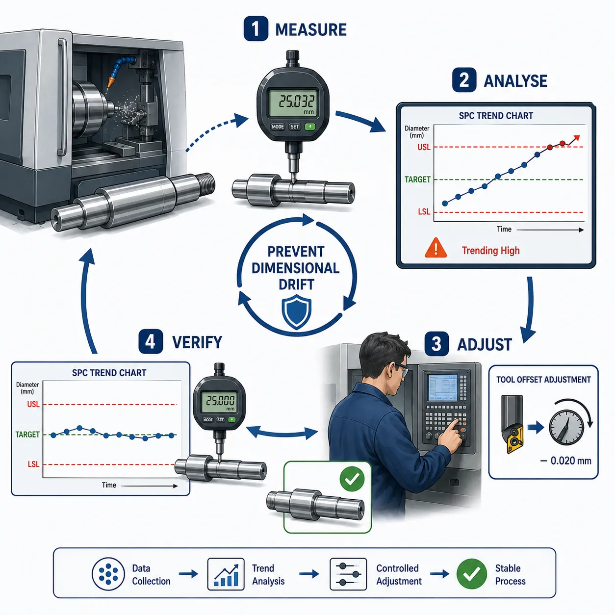
SPC can provide early warning before dimensions become unacceptable.
For example:
Target = 100.00 mm
USL = 100.10 mm
Suppose the process mean moves:
100.01 → 100.03 → 100.05 → 100.07 mm
The process may still be producing acceptable components.
However, continuing without investigation could eventually result in:
100.11 mm
which would exceed the upper specification limit.
Early adjustment can prevent this outcome.
Control Charts for Process Adjustment
Control charts are among the most useful tools for identifying when process adjustment may be justified.
Common charts include:
- X-bar charts.
- R charts.
- Individuals and Moving Range charts.
- p charts.
- np charts.
- c charts.
- u charts.
For dimensional manufacturing, continuous measurements often make X-bar and R charts particularly useful where rational subgroups are available.
X-Bar Chart
An X-bar chart monitors subgroup averages.
It can identify:
- Process mean shifts.
- Gradual movement.
- Unusual subgroup averages.
- Sustained changes.
For example, if five shaft measurements are taken at regular intervals, the average of each subgroup can be plotted over time.
R Chart
An R chart monitors within-subgroup range.
It can identify changes in short-term variation.
This distinction is important.
An X-bar chart may show that the process is moving away from its target.
An R chart may show that the process itself is becoming more variable.
Why Both Charts Matter
Consider two situations.
Situation A: Mean Drift
The X-bar chart shows a gradual upward trend, while the R chart remains stable.
This may indicate:
- Tool wear.
- Offset change.
- Thermal drift.
Situation B: Increasing Variation
The X-bar chart remains approximately centred, while the R chart increases.
This may indicate:
- Machine instability.
- Tool deterioration.
- Fixture inconsistency.
- Material variability.
The corrective approach would therefore be different.
Process Variables and Root Causes
Statistical feedback should not lead directly to random parameter changes.
An engineering team should first identify the likely process mechanism.
For example:
Increasing diameter → inspect tool condition → verify tool wear → confirm offset → review temperature → determine adjustment.
This approach is more reliable than simply changing the machine setting without understanding the cause.
Controlled Process Adjustment
A controlled adjustment should be:
- Technically justified.
- Within authorised operating parameters.
- Documented.
- Traceable.
- Reversible where practical.
- Verified after implementation.
The adjustment should not create new risks.
Examples of Manufacturing Process Adjustments
Tool Offset Adjustment
If a machining process gradually produces oversize components due to predictable tool wear, an approved offset adjustment may restore the process towards its target.
Cutting Parameter Adjustment
If variation is associated with inappropriate cutting conditions, engineers may review:
- Feed rate.
- Cutting speed.
- Depth of cut.
Fixture Adjustment
If dimensional variation is associated with inconsistent workpiece positioning, the fixture may require:
- Realignment.
- Inspection.
- Maintenance.
- Replacement.
Thermal Control
Where dimensional drift is related to temperature, engineers may need to review:
- Machine warm-up.
- Coolant condition.
- Ambient conditions.
- Production sequencing.
Process Adjustment Should Be Based on Evidence
A common quality-control error is adjusting a process after every unusual measurement.
Suppose a shaft measurement is:
50.03 mm
when the target is 50.00 mm.
If the tolerance is ±0.05 mm and the process is statistically stable, this single value may not justify an adjustment.
Frequent unnecessary adjustments can actually increase variation.
This is sometimes referred to as over-adjustment or tampering.
Avoiding Over-Adjustment
An engineer should ask:
- Is the result statistically unusual?
- Is there a trend?
- Is there evidence of a special cause?
- Is the measurement reliable?
- Is the process moving towards a specification limit?
- Is adjustment technically justified?
Only then should an adjustment be considered.
Common-Cause Variation and Adjustment Decisions
If variation is common-cause variation, changing one process variable in response to every fluctuation may make the process less stable.
For example, an operator might adjust a machine after every slightly high measurement.
The result could be:
High value → adjustment → low value → adjustment → high value
This creates additional variation.
The better approach may be to identify and remove the underlying common-cause variation through structured process improvement.
Special-Cause Variation
When a control chart indicates a special cause, investigation becomes appropriate.
Possible causes include:
- Tool breakage.
- Incorrect machine setting.
- Material change.
- Sensor malfunction.
- Fixture damage.
- Unexpected temperature change.
- Maintenance activity.
The process should be investigated before routine production continues.
Process Capability and Adjustment
Process capability indices provide another source of statistical feedback.
Cp assesses potential capability based on spread.
Cpk considers both spread and centring.
If:
Cp is high but Cpk is low
the process may be too close to one specification limit.
This suggests that centring the process may provide the greatest benefit.
If:
Cp and Cpk are both low
the process may have excessive variation.
The engineering response should focus on reducing variation rather than simply moving the process mean.
Practical Example: Shaft Machining
A machining line produces shafts with:
- Target = 50.00 mm.
- LSL = 49.95 mm.
- USL = 50.05 mm.
The process initially produces:
Mean = 50.00 mm.
After extended production, the mean shifts to:
50.03 mm.
The standard deviation remains approximately constant.
The Cpk decreases because the process is closer to the upper specification boundary.
The team investigates tool wear and identifies a predictable dimensional shift.
An approved tool-offset adjustment is introduced.
Post-adjustment measurements show:
Mean = 50.01 mm.
The process is then monitored to confirm stability.
Practical Example: Increasing Variation
A manufacturing process produces components with a target thickness of 10.00 mm.
The specification range is:
9.95–10.05 mm.
The process mean remains near 10.00 mm, but the range between measurements gradually increases.
The R chart indicates increasing variation.
The engineering team investigates:
- Fixture condition.
- Tool condition.
- Material consistency.
- Measurement equipment.
A worn fixture is identified.
After fixture replacement, process variation decreases.
This demonstrates why process adjustment should be linked to the statistical signal.
Practical Example: Thermal Drift
A precision machining process operates continuously for several hours.
Early production measurements are close to target.
Later measurements gradually increase.
The pattern repeats each day.
The engineering team examines production timing and discovers that the dimensional shift corresponds with machine temperature increase.
Possible actions include:
- Controlled warm-up.
- Improved thermal management.
- Coolant-condition control.
- Revised process sequencing.
The objective is to control the underlying thermal influence rather than repeatedly correcting dimensions manually.
Practical Example: Welding Process
A manufacturing line produces welded assemblies.
Statistical analysis identifies gradual changes in a critical weld dimension.
The process team reviews:
- Welding current.
- Voltage.
- Travel speed.
- Consumable condition.
- Joint preparation.
The data indicates that a change in travel speed is associated with dimensional variation.
The process parameter is brought back within its approved range.
The process is then re-monitored.
Process Adjustment Procedure
Step 1: Define the Critical Characteristic
Identify exactly what is drifting.
Examples:
- Diameter.
- Thickness.
- Length.
- Hole position.
- Clearance.
Step 2: Confirm the Specification
Verify:
- Target.
- Upper specification limit.
- Lower specification limit.
- Applicable drawing or technical requirement.
Step 3: Verify Measurement Reliability
Check:
- Calibration.
- Gauge condition.
- Measurement method.
- Resolution.
Step 4: Review Statistical Evidence
Examine:
- Control chart.
- Process mean.
- Standard deviation.
- Range.
- Trend.
- Capability indices.
Step 5: Determine Process Condition
Establish whether the process is:
- Stable.
- Drifting.
- Shifted.
- Increasingly variable.
- Producing special-cause signals.
Step 6: Investigate Potential Causes
Review:
- Tooling.
- Equipment.
- Materials.
- Settings.
- Environment.
- Fixtures.
- Maintenance.
- Operators.
Step 7: Select the Correct Variable
Identify the parameter most directly linked to the observed behaviour.
Step 8: Authorise the Adjustment
Ensure the change complies with:
- Approved procedures.
- Engineering requirements.
- Process limits.
- Safety controls.
Step 9: Implement the Adjustment
Make the controlled change.
Step 10: Verify the Result
Collect additional measurements.
Step 11: Confirm Process Stability
Check whether the statistical behaviour has improved.
Step 12: Update Documentation
Record:
- Original condition.
- Statistical evidence.
- Cause.
- Adjustment.
- Responsible person.
- Date.
- Verification results.
Real-Time Statistical Feedback
Modern manufacturing systems may provide real-time feedback.
Sensors and measurement systems can monitor:
- Dimensional output.
- Temperature.
- Vibration.
- Pressure.
- Speed.
- Torque.
Data can be displayed through:
- Digital dashboards.
- SPC software.
- Automated alerts.
- Process-monitoring systems.
Real-time monitoring can reduce the time between process deterioration and engineering response.
Automated Feedback Systems
Automated systems may be capable of adjusting certain process variables when predefined conditions occur.
For example:
Measurement → Statistical analysis → Threshold detection → Controlled offset adjustment
However, automated adjustment should only operate within appropriately validated and authorised limits.
Benefits of Automated Statistical Feedback
Potential benefits include:
- Faster response.
- Reduced operator dependency.
- Consistent adjustment.
- Reduced dimensional drift.
- Better process repeatability.
- Improved production efficiency.
However, automated feedback requires:
- Reliable sensors.
- Correct algorithms.
- Validated limits.
- Secure control systems.
- Appropriate engineering oversight.
Feedback and Data Quality
Statistical feedback is only as reliable as the data on which it is based.
Potential data-quality problems include:
- Incorrect measurements.
- Calibration errors.
- Missing values.
- Incorrect units.
- Data-entry errors.
- Sensor malfunction.
- Incorrect timestamps.
Before making a significant process adjustment, engineers should confirm that the statistical signal reflects the actual manufacturing process.
Measurement System Analysis
A measurement system should be evaluated for:
- Accuracy.
- Repeatability.
- Reproducibility.
- Resolution.
- Stability.
If measurement variation is too large, it may become difficult to distinguish actual process variation from measurement noise.
Process Adjustment and Traceability
Every significant process adjustment should be traceable.
Useful records include:
- Machine identification.
- Component identification.
- Process parameter.
- Original setting.
- Revised setting.
- Reason for adjustment.
- Statistical evidence.
- Authorisation.
- Verification results.
This allows future engineers to understand why the change occurred.
Feedback From Historical Data
Historical data can reveal recurring process behaviour.
For example, if dimensional drift occurs:
- After 500 production cycles.
- After a particular tool change.
- During high ambient temperatures.
- After a particular material batch.
then the historical pattern can help identify the underlying cause.
Trend Analysis
Trend analysis examines process behaviour over time.
Useful questions include:
- Is the process moving towards a specification limit?
- Is variation increasing?
- Is the process mean shifting?
- Does the pattern repeat?
- Does the change correlate with a known process event?
Run Rules and Statistical Signals
Control charts may use defined statistical rules to identify unusual behaviour.
Signals can include:
- Points outside control limits.
- Long runs on one side of the centre line.
- Sustained upward trends.
- Sustained downward trends.
- Unusual clustering.
The organisation should define the applicable rules within its statistical-control procedure.
Process Adjustment and Preventive Action
The most effective process adjustment can occur before actual non-conformance.
For example:
Process mean moves towards USL → investigate → identify tool wear → controlled offset correction → verify → continue monitoring.
This is preventive process control.
Process Adjustment and Corrective Action
Corrective action may be required after non-conformance has already occurred.
For example:
Out-of-tolerance components detected → production stopped or controlled → root cause investigated → process parameter corrected → affected material assessed → effectiveness verified.
The distinction between preventive adjustment and corrective action should remain clear.
Key Benefits of Statistical Process Adjustment
Prevention of Dimensional Drift
Statistical feedback identifies movement before it reaches specification boundaries.
Reduced Non-Conformance
Early intervention can prevent production of out-of-tolerance components.
Reduced Scrap and Rework
Stable processes reduce unnecessary material waste.
Improved Process Stability
Correctly targeted adjustments can restore predictable behaviour.
Better Equipment Utilisation
Engineers can identify equipment-related drift before major failure.
Improved Product Consistency
Controlled process variables improve dimensional repeatability.
Faster Engineering Response
Real-time data can reduce delays in identifying process changes.
Better QA/QC Integration
Production and quality teams can work from the same statistical evidence.
Improved Maintenance Planning
Repeated process drift may identify equipment maintenance requirements.
Improved Cost Control
Reducing defects lowers the cost associated with rework, scrap and inspection.
Common Errors in Process Adjustment
Adjusting After Every Measurement
Individual fluctuations may be normal.
Ignoring Trends
A process can remain within specification while becoming increasingly unstable.
Adjusting Without Root-Cause Investigation
Random changes can introduce additional variation.
Using Incorrect Control Limits
Control limits should be calculated using appropriate statistical methods.
Confusing Specification Limits With Control Limits
They represent different concepts.
Ignoring Measurement Errors
A false signal can result in an unnecessary adjustment.
Making Unauthorised Parameter Changes
Process changes should follow controlled procedures.
Failing to Verify Adjustments
An adjustment is not successful simply because the machine setting changed.
Ignoring Long-Term Behaviour
Short-term improvement may not represent sustainable control.
Case Study: Statistical Control of a Precision Turning Process
Background
A manufacturing organisation produces precision shafts used in industrial mechanical assemblies.
The required diameter is:
50.00 ± 0.05 mm.
The process initially operates close to target.
Initial Monitoring
The QA/QC team establishes an X-bar and R chart using rational subgroups.
The process is initially stable.
The mean is:
50.00 mm.
The standard deviation remains low.
Emerging Trend
After several production periods, the X-bar chart shows a gradual upward trend.
The R chart remains relatively stable.
The process mean reaches:
50.03 mm.
Although all components remain within specification, the trend indicates potential drift.
Investigation
The engineering team reviews:
- Tool condition.
- Machine offsets.
- Spindle temperature.
- Coolant.
- Fixture condition.
- Maintenance records.
Tool wear is found to be increasing gradually.
Adjustment
An approved tool-offset adjustment is introduced.
The process mean returns closer to:
50.01 mm.
Verification
The team collects additional data and confirms:
- No unusual control-chart signals.
- Stable range.
- Improved process centring.
- Reduced risk of approaching the upper specification limit.
Long-Term Action
The organisation introduces a tool-condition monitoring strategy.
Instead of waiting for excessive dimensional drift, the team uses statistical feedback to establish an appropriate intervention point.
Outcome
The manufacturing process becomes more predictable, while unnecessary premature tool replacement is avoided.
Advanced Case Study: Multiple Variable Interaction
A complex machining line produces a precision housing.
The measured bore diameter begins to drift.
Initial investigation suggests tool wear.
However, historical data shows that the dimensional shift is stronger during longer production runs.
Further analysis identifies:
- Tool wear.
- Machine temperature.
- Coolant condition.
The engineering team does not change one parameter immediately.
Instead, it analyses the relationship between:
- Operating time.
- Temperature.
- Tool condition.
- Bore diameter.
The evidence shows that thermal effects contribute significantly to the drift.
The corrective strategy therefore combines:
- Thermal stabilisation.
- Tool-condition monitoring.
- Controlled offset adjustment.
This demonstrates the importance of understanding interacting process variables.
Management of Process Changes
When process variables are changed, the organisation should control:
- Authorisation.
- Documentation.
- Technical justification.
- Safety implications.
- Quality implications.
- Verification.
- Change history.
Uncontrolled process changes can create hidden variation and make future statistical analysis difficult.
Change Control
A significant process change should be evaluated before implementation.
Questions may include:
- What variable is being changed?
- Why is it being changed?
- What evidence supports the change?
- What are the expected effects?
- Could other characteristics be affected?
- What verification is required?
- What happens if the change is unsuccessful?
Verification After Adjustment
Verification should confirm that:
- The target has been restored where appropriate.
- Variation remains controlled.
- No new defect has emerged.
- The process remains stable.
- Capability has improved or remained acceptable.
A single measurement after adjustment is generally insufficient to establish sustained process improvement.
Re-establishing the Process Baseline
Following a significant process change, engineers may need to establish a new baseline.
The baseline may include:
- Mean.
- Standard deviation.
- Control limits.
- Capability indices.
- Normal operating parameters.
The new baseline should be documented and controlled.
Statistical Feedback and Continuous Improvement
Statistical feedback supports continual improvement through a structured cycle:
Measure
Collect reliable process data.
Analyse
Use statistical methods to understand variation.
Interpret
Determine whether the process is stable, drifting or changing.
Investigate
Identify likely causes.
Adjust
Modify the appropriate process variable within controlled limits.
Verify
Confirm that the adjustment achieved the intended result.
Standardise
Update the process where the improvement is confirmed.
Monitor
Continue statistical monitoring to ensure sustainability.
Professional Engineering Judgement
Statistical feedback does not remove the need for professional judgement.
Engineers should consider:
- Mechanical function.
- Safety.
- Equipment condition.
- Product criticality.
- Production requirements.
- Design tolerances.
- Measurement reliability.
- Process capability.
- Cost implications.
A process adjustment that improves one dimension but adversely affects another characteristic may not represent genuine improvement.
Balancing Quality and Production Efficiency
Process adjustments should avoid unnecessary production disruption.
For example, stopping a production line for every minor statistical fluctuation may reduce productivity without improving quality.
Conversely, ignoring strong statistical signals may result in significant scrap and rework.
The correct balance involves:
- Defined statistical rules.
- Risk-based intervention.
- Controlled response procedures.
- Engineering judgement.
Integrating Statistical Feedback With Maintenance
Process drift can provide an early indication of equipment deterioration.
For example:
Increasing dimensional variation → possible spindle deterioration → engineering inspection → maintenance intervention → restored process stability.
This allows quality data to support predictive and preventive maintenance.
Integrating Statistical Feedback With Supplier Materials
Incoming material variation can also influence production dimensions.
For example:
Material hardness increases → cutting response changes → dimensional drift develops.
Statistical feedback may therefore require collaboration between:
- Production.
- QA/QC.
- Maintenance.
- Engineering.
- Procurement.
- Suppliers.
Digital Manufacturing Applications
Advanced manufacturing environments may combine SPC with:
- Automated measurement.
- Machine sensors.
- Manufacturing execution systems.
- Digital dashboards.
- Statistical software.
- Automated alerts.
These systems can create faster feedback loops.
However, engineers should ensure that:
- Data sources are validated.
- Algorithms are appropriate.
- Control limits are correctly established.
- Changes are authorised.
- Records are traceable.
Practical Engineering Decision Framework
When statistical feedback identifies potential dimensional drift, engineers can use the following sequence:
- Confirm the measurement.
- Check the control chart.
- Review the process trend.
- Confirm specification requirements.
- Determine whether the signal is statistically meaningful.
- Check for special causes.
- Review machine and tooling condition.
- Identify the most likely process variable.
- Determine an appropriate adjustment.
- Implement the controlled change.
- Collect verification data.
- Confirm stability.
- Review capability.
- Document the result.
- Continue monitoring.
Conclusion
Adjusting manufacturing process variables based on statistical feedback is a critical component of modern mechanical engineering quality control. Manufacturing processes naturally experience variation, but systematic statistical monitoring enables engineering teams to distinguish expected process behaviour from meaningful changes that could lead to dimensional drift. Control charts, process capability indices, trend analysis, standard deviation, subgroup analysis, and historical production data provide objective evidence for determining when investigation or adjustment may be required.
Effective process adjustment is not simply a matter of changing machine settings whenever a measurement moves away from the target. Engineers must first confirm measurement reliability, examine statistical evidence, distinguish common-cause variation from special-cause variation, identify likely physical causes, and determine whether intervention is justified. Unnecessary adjustment can create additional variation, while delayed intervention can allow a stable process to drift towards specification limits. The objective is therefore controlled intervention based on reliable evidence.
When an appropriate process variable is identified, the adjustment should be implemented within authorised engineering limits and followed by verification. Post-adjustment data should demonstrate that the process has returned to a stable and acceptable condition without creating new problems elsewhere. Capability analysis can then confirm whether the process remains capable of meeting design tolerances. Documentation and traceability ensure that the adjustment, technical justification, and verification evidence are retained for future quality and engineering review.
The integration of statistical feedback with manufacturing control, equipment maintenance, QA/QC inspection, measurement-system management, and continual improvement creates a proactive quality-control environment. It enables organisations to detect dimensional drift early, reduce scrap and rework, improve process stability, optimise equipment performance, and maintain consistent mechanical component quality. Most importantly, it transforms production data into practical engineering intelligence, allowing manufacturing processes to be controlled before variation develops into significant non-conformance, reliability problems, or operational disruption.